Chapter 4 Trigonometry
4.1 Pythagoras
The most fundamental result in trigonometry is the Pythagorean Theorem:
Theorem 4.1 (Pythagorean Theorem) In a right-angle triangle, the hypotenuse is the side opposite the right angle.
In any right-angle triangle, the square of the hypotenuse is equal to the sum of the squares of the other two sides.
With reference to figure 4.1, we have
\[c^2=a^2+b^2\]

Figure 4.1: A right-angled triangle with sides \(a, b\) and \(c\), with \(c\) being the hypotenuse.
One particular application is finding the distance between two points in a Cartesian coordinate system.
4.2 Degrees and radians
We can measure an angle in two different units: degrees or radians.
In degrees, we split a full circle into 360 segments and then call the angle bewteen each segment 1 degree, or \(1^\circ\). Of course a full circle is \(360^\circ\).
An alternative measure of angle is radians. In this case, we start from the fact that the circumference of a circle is given by \[ C=2\pi r \] where \(r\) is the radius of the circle. If we had a circle with radius \(r=1\), then the circumference is \(C=2\pi\). Now we consider this circle to be split into \(2\pi\) segments7, with each segment being 1 radian, or \(1 \text{ rad}\). A full circle is then \(2\pi \text{ rad} = 6.283 \text{ rad}\) (to 3 d.p.).
Sometimes it is more convenient to work in degrees, and other times it is more convenient to work in radians. We can easily convert between degrees and radians as follows. If we have an angle \(D^\circ\) in degrees, then the corresponding angle in radians \(R \text{ rad}\) is: \[ R \text{ rad}=\frac{2\pi}{360}\times D^\circ \] and in the other direction \[ D^\circ=\frac{360}{2\pi}\times R \text{ rad}. \]
Where possible, we would state radians as multiples of \(\pi\), so in particular:
| Degrees | Radians |
|---|---|
| \(360^\circ\) | \(2\pi\text{ rad}\) |
| \(270^\circ\) | \(\frac{3}{2}\pi\text{ rad}\) |
| \(180^\circ\) | \(\pi\text{ rad}\) |
| \(120^\circ\) | \(\frac{2}{3}\pi\text{ rad}\) |
| \(90^\circ\) | \(\frac{\pi}{2}\text{ rad}\) |
| \(60^\circ\) | \(\frac{\pi}{3}\text{ rad}\) |
| \(45^\circ\) | \(\frac{\pi}{4}\text{ rad}\) |
| \(30^\circ\) | \(\frac{\pi}{6}\text{ rad}\) |
Note that a scientific calculator will have a button to switch between using degrees and radians: make sure your calculator is in the correct mode!
4.3 Trigonometric ratios
Calculating angles and side lengths of right-angled triangles is of fundamental importance in science and engineering applications.

Figure 4.2: A right-angled triangle.
Recall that we can calculate relationships between angles and side lengths of a right-angled triangle (as described in figure 4.2) using sine, cosine and tangent:
\[\begin{align*} \sin(\theta)&=\frac{Opp.}{Hyp.}\\ \cos(\theta)&=\frac{Adj.}{Hyp.}\\ \tan(\theta)&=\frac{Opp.}{Adj.} \end{align*}\]
A useful way to remember these relationships is the mnemonic “SOH CAH TOA”:
SOH - Sine equals Opposite over Hypotenuse
CAH - Cosine equals Adjacent over Hypotenuse
TOA - Tan equals Opposite over Adjacent
These are most commonly used to determine angles by using the inverse functions:
\[\begin{align*} \theta&=\sin^{-1}(\frac{Opp.}{Hyp.})\\ \theta&=\cos^{-1}(\frac{Adj.}{Hyp.})\\ \theta&=\tan^{-1}(\frac{Opp.}{Adj.}) \end{align*}\]
WARNING: the notation suggests we are taking \(\sin\) to the power \(-1\), so that \(\sin^{-1}=\frac{1}{\sin}\), but this is NOT how the inverse is defined. Remember that the inverse “undoes” the action of the function. Scientific calculators will have buttons to apply these functions. The inverses are also sometimes called
\[\begin{align*} \arcsin&=\sin^{-1},\\ \arccos&=\cos^{-1},\\ \arctan&=\tan^{-1}. \end{align*}\]
Example 4.1 (Applying inverse trig. functions) Calculate the angle \(\theta\) in the following triangle.

Figure 4.3: A right angled triangle with hypotenuse legth 14 units and adjacent length 8 units.
Since we have the lengths of the hypotenuse and adjacent, we can use \(\cos^{-1}\) to find \(\theta\). Using a calculator we find
\[\theta=\cos^{-1}\left(\frac{8}{14}\right)=55.15^\circ \text{(to 2 d.p.)}\]
We also have special names for the reciprocal trigonometric functions:
\[\begin{align*} \operatorname{cosec}(\theta)&=\frac{1}{\sin(\theta)},\\ \sec(\theta)&=\frac{1}{\cos(\theta)},\\ \cot(\theta)&=\frac{1}{\tan(\theta)}. \end{align*}\]
4.4 Sine and cosine rules
The Pythagorean Theorem and Trigonometric ratios above only apply to right-angle triangles. For general triangles, the sine and cosine rules give us useful relationsips between angles and side lengths.

Figure 4.4: A general triangle with angles \(A, B,\) and \(C\) and the corresponding opposite sides as \(a, b\) and \(c\).
Theorem 4.2 (Sine Rule) Label a triangle with angles \(A, B,\) and \(C\) and the corresponding opposite sides as \(a, b\) and \(c\) (as in figure 4.4). Then,
\[\frac{a}{\sin(A)}=\frac{b}{\sin(B)}=\frac{c}{\sin(C)}.\]
This is useful when we have:
- one side and any two angles, or
- two sides and an angle (but not the included angle).
Theorem 4.3 (Cosine Rule) Label a triangle with angles \(A, B,\) and \(C\) and the corresponding opposite sides as \(a, b\) and \(c\) (as in figure 4.4). Then,
\[\begin{align*} a^2&= b^2 +c^2 -2bc\cos(A)\quad\text{ or,}\\ b^2&=a^2+c^2-2ac\cos(B)\quad\text{ or,}\\ c^2&=a^2+b^2-2ab\cos(C). \end{align*}\]
This is useful when we have:
- two sides and the included angle, or
- three sides.
4.5 Angles in Cartesian Coordinates
When calculating angles in the Cartesian plane we need to be a bit careful with the inverse trigonometric functions, because they are only directly valid in certain ranges (see section @ref(inverse_trig_funcs)). The easiest way around this is to always find a suitable right-anged triangle, and then interpret the angles and lengths correctly in the plane (as we will show below). We usually measure angles in the Cartesian plane from the positive \(x\)-axis in an anti-clockwise direction. Negative angles correspond to measuring in the clockwise direction, so that, for example: \(180^\circ\) is equivalent to \(-180^\circ\), \(90^\circ\) is equivalent to \(-270^\circ\), etc. Also, angles greater than \(360^\circ\), or \(2\pi\text{ rad}\), correspond to “wrapping” around the circle more than once, for example: \(360^\circ\) is equivalent to \(0^\circ\), \(405^\circ\) is equivalent to \(45^\circ\), \(-540^\circ\) is equivalent to \(180^\circ\).
Let’s consider a circle centered at the origin, which has equation \(x^2+y^2=r^2\), where \(r\) is the radius (note that by Pythagoras this equation is all points that are a distance \(r\) from the origin).
What is the angle between the \(x\)-axis and a radial line joining the origin \((0,0)\) to a point \((x,y)\) on the circle? Let’s first assume \(x\) and \(y\) are positive. We can consider a triangle formed from the points \((0,0)\), \((x,y)\) and \((x,0)\). Then we know the hypotenuse has length \(r\), the opposite has length \(y\) and the adjacent has length \(x\), and since we have a right-angled triangle we can use all of the usual trigonometric ratios to calculate angles and lengths in this triangle.
Now consider a point \((x,y)\) with \(x\) negative and \(y\) positive, that is, in the second quadrant. We can draw a right-angled triangle between the points \((0,0)\), \((x,0)\) and \((x,y)\). Since we want to consider lengths in this triangle, we take the positive value \(|x|\). Then the angle \(\phi\) between the negative \(x\)-axis and the radial line can be found from \(\phi = \arctan\left(\frac{y}{|x|}\right)\). However, the actual angle we want is \(\theta\), and so we can get this from \(\theta = 180^\circ - \phi\), or in radians \(\theta=\pi-\phi\). We can do a similar proceedure in the remaining two quadrants.
4.6 Trigonometric waveforms
The trigonometric functions often arise in applications in the context of waves. Whilst there are different forms of waves, trigonometric waves are arguably the most ubiquitous.
In general, a function of the form \[ f(x)=A\sin(\omega x + \phi) \] with parameters \(A,\omega\) and \(\phi\) is known as a sinusoidal function.
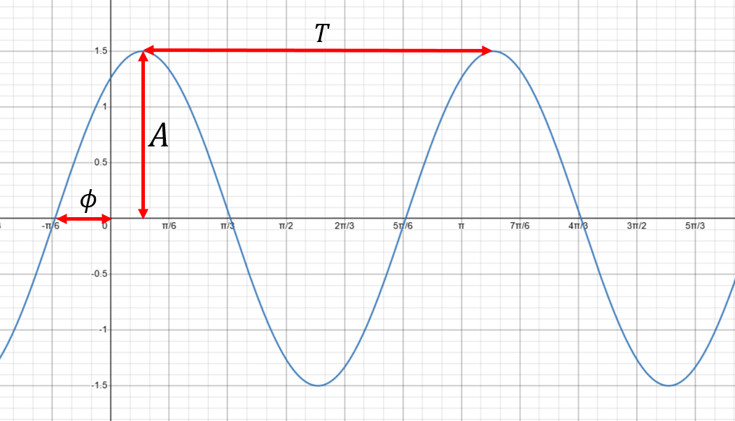
Figure 4.5: A sinusoidal wave form plotted in radians.
- \(A\) is called the amplitude – this determines the range of values, from \(-A\) to \(A\);
- \(\omega\) is the angular frequency – the rate of change of the sine function argument in units of radians per second or degrees per second;
- \(\phi\) is the phase – this determines the offset of the sine function at \(x=0\) in units of radians or degrees.
- \(T=\frac{2\pi}{\omega}\) is the length of one cycle e.g. measured from peak to peak, or trough to trough. If \(x\) represents time, then \(T\) is called the period. If \(x\) represents distance, then \(T\) is usually denoted by \(\lambda\) and called the wavelength.
Figure 4.6: The function \(f(x)=A\sin(\omega x + \phi)\) (blue curve). [Open graph in browser.]
A useful formula for combining \(\sin\) and \(\cos\) waves is:
\[a\cos(\theta)+b\sin(\theta)=R\cos(\theta-\phi)\]
where:
\(R=\sqrt{a^2+b^2}\)
\(\phi=\tan^{-1}(b/a)\)
Such waves are associated with circular motion. If we imagine a particle moving around a circle at a constant angular speed and take the projection onto one of the coordinate axes, for example the \(y\)-axis, then the displacement from the origin plotted against time will draw out a sinusoid. This is becuase the position on the \(y\)-axis is \(y=r\sin(\theta)\).
(#fig:circular_motion)Click the play button in block 1 (next to variable \(t\), the angle). Demonstration of a sinusoidal wave from circular motion: as the angle \(t\) increases and the point moves around the circle (red) the projection onto the \(y\) axis (blue) describes a sinusoid (green). [Open graph in browser.]
4.7 Trigonometric identities
Recall that there are a number of useful relationships between the trigonometric functions. Here are some key ones.
4.7.1 Pythagorean identities
These follow from the Pythagorean theorem.
\[\begin{gather*} \sin^2(\theta)+\cos^2(\theta)=1\\ 1+\tan^2(\theta)=\sec^2(\theta)\\ \cot^2(\theta)+1=\operatorname{cosec}^2(\theta) \end{gather*}\]
4.7.2 Compound angle formulae
The following formulae allow us to manipulate sines, cosines and tangents of the sum or difference of two angles.
\[\begin{align*} \sin(\theta+\phi)&=\sin(\theta)\cos(\phi)+\cos(\theta)\sin(\phi)\\ \sin(\theta-\phi)&=\sin(\theta)\cos(\phi)-\cos(\theta)\sin(\phi)\\ \cos(\theta+\phi)&=\cos(\theta)\cos(\phi)-\sin(\theta)\sin(\phi)\\ \cos(\theta-\phi)&=\cos(\theta)\cos(\phi)+\sin(\theta)\sin(\phi)\\ \tan(\theta+\phi)&=\frac{\tan(\theta)+\tan(\phi)}{1-\tan(\theta)\tan(\phi)}\\ \tan(\theta-\phi)&=\frac{\tan(\theta)-\tan(\phi)}{1+\tan(\theta)\tan(\phi)} \end{align*}\]
4.7.3 Double angle formulae
Setting \(\phi=\theta\) in the compound angle formulae gives the following double angle formulae:
\[\begin{align*} \sin(2\theta)&=2\sin(\theta)\cos(\theta)\\ \cos(2\theta)&=\cos^2(\theta)-\sin^2(\theta)\\ \tan(2\theta)&=\frac{2\tan(\theta)}{1-\tan^2(\theta)} \end{align*}\]
4.7.4 Product to sum formulae
From the compound angle formulae we can derive the following.
\[\begin{align*} \sin(\theta)\cos(\phi)&=\frac{1}{2}[\sin(\theta+\phi)+\sin(\theta-\phi)]\\ \cos(\theta)\sin(\phi)&=\frac{1}{2}[\sin(\theta+\phi)-\sin(\theta-\phi)]\\ \cos(\theta)\cos(\phi)&=\frac{1}{2}[\cos(\theta+\phi)+\cos(\theta-\phi)]\\ \sin(\theta)\sin(\phi)&=-\frac{1}{2}[\cos(\theta+\phi)-\cos(\theta-\phi)]\\ \end{align*}\]
4.7.5 Sum to product formulae
In the other direction (also derived from the compound angle formulae) we have the following.
\[\begin{align*} \sin(\theta)+\sin(\phi)=2\sin\left(\frac{\theta+\phi}{2}\right)\cos\left(\frac{\theta-\phi}{2}\right)\\ \sin(\theta)-\sin(\phi)=2\cos\left(\frac{\theta+\phi}{2}\right)\sin\left(\frac{\theta-\phi}{2}\right)\\ \cos(\theta)+\cos(\phi)=2\cos\left(\frac{\theta+\phi}{2}\right)\cos\left(\frac{\theta-\phi}{2}\right)\\ \cos(\theta)-\cos(\phi)=-2\sin\left(\frac{\theta+\phi}{2}\right)\sin\left(\frac{\theta-\phi}{2}\right) \end{align*}\]
Note this is not an integer number of segments! It is approximately 6.283 segments.↩︎