Chapter 21 Continuous Random Variables
Recall that a random variable is a numerical valued function defined on the sample space. In plain language, it is a rule for assigning a number to each point in the sample space.
So far all our discussion has been about discrete random variables i.e. those whose range of values is finite or countably infinite. However, it is conceptually possible for a random variable to take a continuum of values, such as an interval of real values (or a number of such intervals).
A continuous random variable has an uncountably infinite number of possible values.
Most properties of continuous random variables are analogous to the ideas we have already seen for discrete random variables, but the probability mass function is replaced by the probability density function, and summation is replaced by integration.
Consider the random variable \(X\) which represents the life, in hours, of a 100 watt electric light bulb. The range of values of \(X\) is the interval \(0 \leq x < \infty\), which is not a countably infinite set. So \(X\) is a continuous random variable. Suppose that \(a\) and \(b\) are two non-negative real values with \(a < b\), then \({a \leq X \leq b}\) is an event in the sample space of \(X\), so we should be able to define the probability, \(P(a \leq X \leq b)\), that this event occurs.
In general for a continuous random variable we assume there is some function \(f_X(x)\), such that for all \(a < b\): \[ P(a \leq X \leq b) = \int_a^b f_X(x) dx. \] We call the function \(f_X(x)\) the probability density function of the continuous random variable \(X\). Hence \(P(a \leq X \leq b)\) is equal to the area under the graph of \(f_X(x)\) between \(x = a\) and \(x = b\).
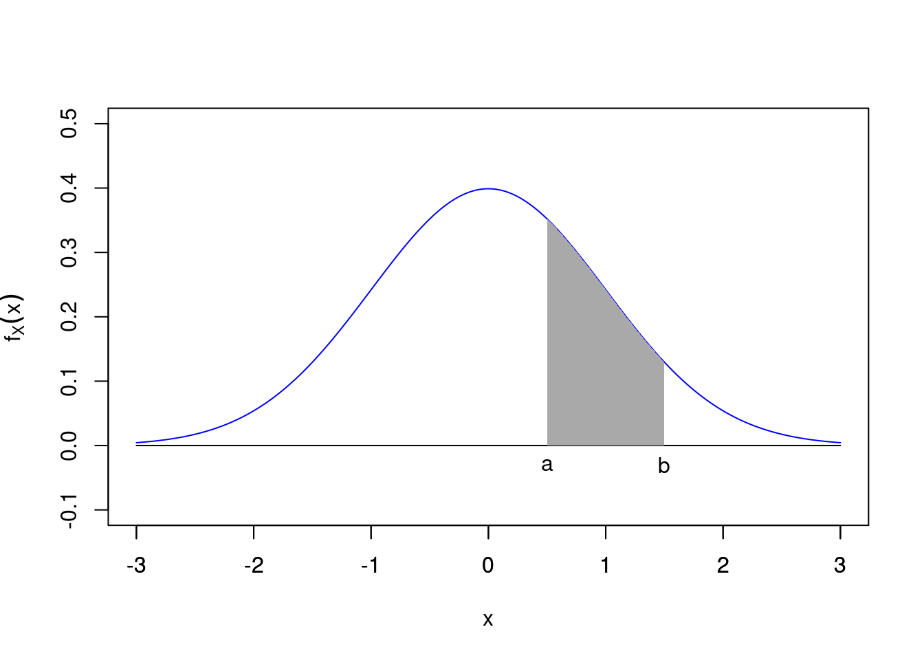
Figure 21.1: \(P(a<X<b)\) is the area under \(f_X(x)\) from \(a\) to \(b\)
When the range of values of a random variable is a continuum, we concentrate on probabilities of events such as \(a \leq X \leq b\), rather than events such as \(X = a\). We can see that: \[P(X = a) = \int_a^a f_X(x) dx =0.\] Hence if \(X\) is a continuous random variable then for any single real number \(a\), \(P(X = a) = 0\). (Note \(P(X=a)\neq f_X(a)\), since \(f_X\) is a probability density not a probability.) This also means we do not in general have to distinguish between \(P(a < X)\) and \(P(a \leq X)\) or between \(P(X < b)\) and \(P(X \leq b)\) for continuous random variables.
As with discrete random variables, the probability of the whole sample space for a continuous random variable must be one, so \(f_X(x)\) must integrate to one over the range of \(X\) i.e.: \[ \int_{-\infty}^{\infty} f_X(x) = 1. \] Note we can take this integral to be over the whole real line \((-\infty, \infty)\), since even if the range of possible values of \(X\) is more restricted than that, then \(f_X(x)\) will be zero outside of its range.
21.1 Uniform distribution
A random variable \(X\) is equally likely to take any value in the range \([a, b]\), where \(a < b\). What is the probability density function of \(X\)?
If \(X\) is equally likely to take any value in the range \([a, b]\), then the probability density function of \(X\) must be a constant across the range. Hence, \(f_X(x) = c\) for some \(c > 0\) when \(x \in [a, b]\).
Since \(\int_a^b c~dx = 1\), then this implies that \(c = 1 / (b - a)\). Hence, \[ f_X(x) = \begin{cases} \frac{1}{b - a} & \mbox{for $x \in [a, b]$,}\\ 0 & \mbox{otherwise.} \end{cases}. \] Here \(X \sim U(a, b)\) has a uniform distribution.
As an example, we plot the probability density function for \(X \sim U(-0.5, 1.5)\).
\[ f_X(x) = \begin{cases} \frac{1}{2} & \mbox{for $-0.5 < x < 1.5$,}\\ 0 & \mbox{otherwise.} \end{cases}. \]
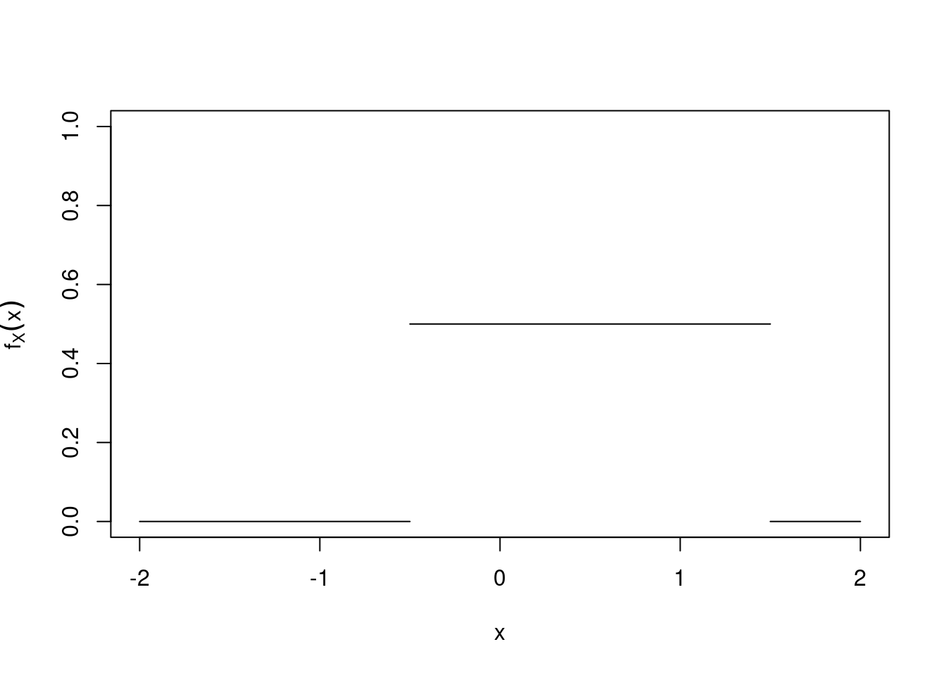
Figure 21.2: Graph of the density function \(f_X(x)\) for \(X\sim U(-0.5,1.5)\).
21.2 Cumulative Distribution Function
For a continuous random variable \(X\), we define the cumulative distribution function of \(X\) in a similar way to that for a discrete random variable i.e: \[ F_X(x) = P(X < x) = \int_{-\infty}^{x} f_X(u) du. \] Note that, as for discrete random variables, if \(X\) is continuous then \(0 \leq F_X(x) \leq 1\) (because \(F_X(x)\) is a probability).
Furthermore, \(F_X(x)\) is a non-decreasing function of \(x\), with \[ \lim_{x \to -\infty} F_X(x) = 0 \quad \mbox{and} \quad \lim_{x \to \infty} F_X(x) = 1. \]
In the continuous case \(F_X(x)\) is in general a smooth (usually S shaped) curve rather than a step function as it is in the discrete case. \(F_X(x)\) is defined for all values of \(x\) (not just the range of values for which \(f_X(x)\) is non-zero).
For example, if \(X \sim U(a, b)\), then \[ F_X(x) = \begin{cases} 0 & \mbox{for $x < a$,}\\ \frac{x - a}{b - a} & \mbox{for $a < x < b$,}\\ 1 & \mbox{for $x > b$.} \end{cases}. \]
As an example, we plot the cumulative distribution function for \(X \sim U(-0.5, 1.5)\).
\[ F_X(x) = \begin{cases} 0 & \mbox{for $x < -0.5$,}\\ \frac{x + 0.5}{2} & \mbox{for $-0.5 < x < 1.5$,}\\ 1 & \mbox{for $x > 1.5$.} \end{cases}. \]
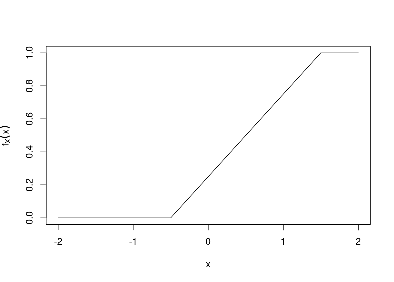
Figure 21.3: Graph of the cumulative distribution function \(F_X(x)\) for \(X\sim U(-0.5,1.5)\).
The distribution function is useful for calculating probabilities such as \(P(a \leq X \leq b)\), since \[ P(a \leq X \leq b) = P(X \leq b) - P(X \leq a) = F_X(b) - F_X(a). \]
21.3 Expectation and Variance
The expected value of a continuous random variable \(X\) is: \[ \operatorname{E}(X) = \int_{-\infty}^{\infty} xf_X(x) dx. \] Remember that if the range of values of \(X\) is more restricted than the whole real line, then \(f_X(x)\) will be zero outside of this range, so this definition still holds. In essence we say that we “integrate over the range of values” of \(X\). This is analogous to the discrete case, except we take an integral instead of a sum.
Example 21.1 (Expectation of a Uniform RV) If \(X \sim U(a, b)\), what is \(\operatorname{E}(X)\)?
\[\begin{eqnarray*} \operatorname{E}(X) = \int_{a}^{b} \frac{x}{b - a} dx &=& \left[\frac{x^2}{2(b - a)} \right]_{a}^{b} \\ &=& \frac{b^2 - a^2}{2(b - a)} \\ &=& \frac{(b - a)(b + a)}{2(b - a)}\\ &=& \frac{b+a}{2}. \end{eqnarray*}\]
The variance of a continuous random variable \(X\) is defined in the same way as for the discrete case: \[ \operatorname{var}(X) = \operatorname{E}\left([X - \operatorname{E}(X)]^2\right) = \int_{-\infty}^{\infty} (x - \mu)^2f_X(x) dx, \] where \(\mu = \operatorname{E}(X)\).
Other analogous properties to the discrete case also hold:
Let \(a\) and \(b\) be constants, and let \(g(X)\) and \(h(X)\) be functions defined on the range of a random variable \(X\). Then, \[ \operatorname{E}\left[ag(X) + bh(X)\right] = a\operatorname{E}[g(X)] + b\operatorname{E}[h(X)] \] and in particular \(\operatorname{E}(aX + b) = a\operatorname{E}(X) + b\).
If \(g(\cdot)\) is a function of a continuous random variable \(X\), then: \[ E\left[g(X)\right] = \int_{-\infty}^{\infty} g(x)f_X(x) dx. \]
It can be shown that \[ \operatorname{var}(X) = E\left(X^2\right) - E^2(X), \] and \(\operatorname{var}(aX + b) = a^2\operatorname{var}(X)\).
Example 21.2 (Variance of a Uniform RV) If \(X \sim U(a, b)\), what is \(\operatorname{var}(X)\)?
We can calculate \[\begin{eqnarray*} \operatorname{E}\left(X^2\right) = \int_{a}^{b} \frac{x^2}{b - a} dx &=& \left[\frac{x^3}{3(b - a)} \right]_{a}^{b} \\ &=& \frac{b^3 - a^3}{3(b - a)}. \end{eqnarray*}\] Hence, \[\begin{eqnarray*} \operatorname{var}(X) = E\left(X^2\right) - E^2(X) &=& \frac{b^3 - a^3}{3(b - a)} - \frac{(a + b)^2}{4}\\ &=& \frac{(b - a)^2}{12}. \end{eqnarray*}\]
21.4 Normal Distribution
The normal (or ) distribution is the king of probability distributions.
We say that \(X\) has the standard normal distribution if its density function is \[ \phi(x)=\frac{e^{-x^2/2}}{\sqrt{2\pi}} \] for \(-\infty < x < \infty\). The graph of \(\phi\) is the famous “bell-shaped curve”.
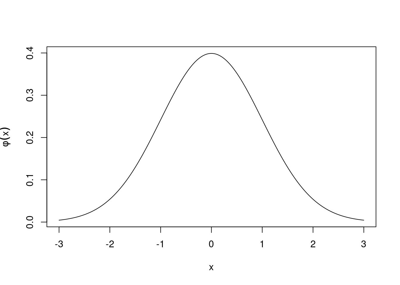
Figure 21.4: Graph of the normal distribution density function \(\phi\).
If \(\phi\) is a density, we should have \[ \frac{1}{\sqrt{2\pi}}\int_{-\infty}^\infty e^{-x^2/2}\,dx = 1. \] However, evaluating this definite integral requires methods beyond the scope of these notes.
The mean and variance are \(\operatorname{E}(X)=0\) and \(\operatorname{var}(X)=1\).
If \(X\) is a standard normal random variable and \(Y=\sigma X+\mu\) where \(\sigma>0\) and \(-\infty < \mu < \infty\), then \(Y\) has a normal (Gaussian) distribution with mean \(\mu\) and variance \(\sigma^2\).
The probability density function of \(Y\) is \[ f_Y(y)=\frac1{\sigma\sqrt{2\pi}}\exp\left[-\frac{(y-\mu)^2}{2\sigma^2}\right]. \] We write \(Y\sim N(\mu,\sigma^2)\) to denote the distribution of this random variable being a normal distribution with mean \(\mu\) and variance \(\sigma^2\). The plot is shifted to the right by \(\mu\) and “stretched” by \(\sigma\).
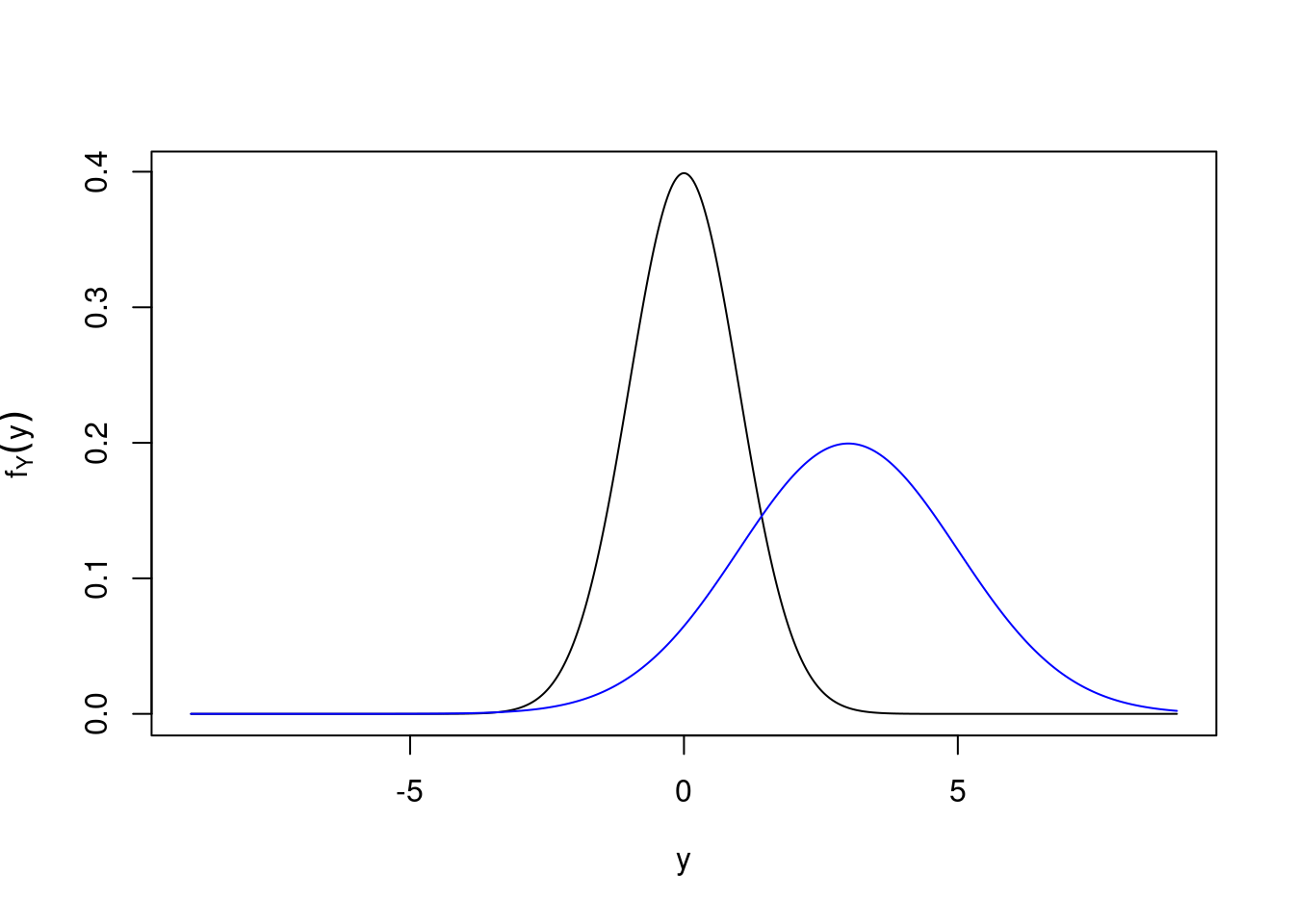
Figure 21.5: Density for \(Y\sim N(3,4)\).
The cumulative distribution function of a standard normal random variable, usually denoted by \(\Phi\), is \[ \Phi(x)=P(X < x)=\frac1{\sqrt{2\pi}}\int_{-\infty}^x e^{-u^2/2}\,du \] but this integral can’t be expressed in terms of standard functions, like exponentials, logarithms and trigonometric functions. For this reason, values of this function (\(\Phi(x)\)) are tabulated in statistical tables (but usually not available on pocket calculators).
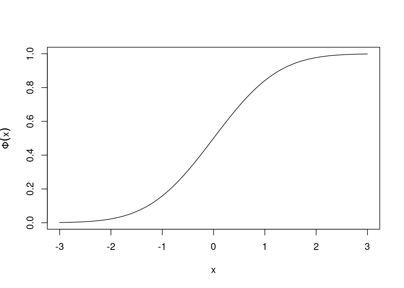
Figure 21.6: Cumulative distribution function \(\Phi(x)\).
We remark on one useful identity. Since the standard normal distribution is symmetric about zero \[\begin{eqnarray*} \Phi(-x)&=&P(X < -x)=P(X > x)\\ &=&1-P(X < x)=1-\Phi(x) \end{eqnarray*}\] and it’s only necessary to tabulate \(\Phi(x)\) for \(x>0\).
21.5 Standard Normal Distribution Tables
There are two forms commonly used, tabulating either .
\[P(X<x)=\int_{-\infty}^x \phi(u)\,du$=\Phi(x)\] or \[P(0<X<x)=\int_{0}^x \phi(u)\,du=\Phi(x)-\Phi(0)=\Phi(x)-0.5\] where \(X\sim N(0,1)\) and noting \(\Phi(0)=0.5\) by symmetry. To save space, values of \(P(X< x)\) or \(P(0< X < x)\) are listed down the rows in increments of \(x\) by \(0.1\) and along the columns in increments of \(x\) by \(0.01\).
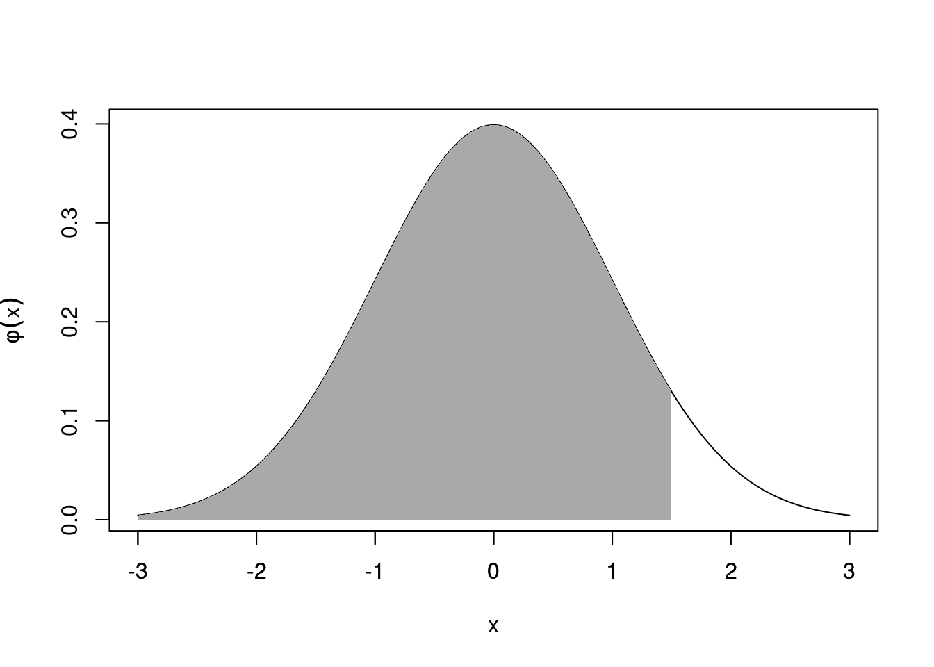
Figure 21.7: \(P(X<x)\) is the area under \(\phi(x)\) from \(-\infty\) to \(x\)
| 0 | 0.01 | 0.02 | 0.03 | 0.04 | 0.05 | 0.06 | 0.07 | 0.08 | 0.09 | |
|---|---|---|---|---|---|---|---|---|---|---|
| 0 | 0.5000 | 0.5040 | 0.5080 | 0.5120 | 0.5160 | 0.5199 | 0.5239 | 0.5279 | 0.5319 | 0.5359 |
| 0.1 | 0.5398 | 0.5438 | 0.5478 | 0.5517 | 0.5557 | 0.5596 | 0.5636 | 0.5675 | 0.5714 | 0.5753 |
| 0.2 | 0.5793 | 0.5832 | 0.5871 | 0.5910 | 0.5948 | 0.5987 | 0.6026 | 0.6064 | 0.6103 | 0.6141 |
| 0.3 | 0.6179 | 0.6217 | 0.6255 | 0.6293 | 0.6331 | 0.6368 | 0.6406 | 0.6443 | 0.6480 | 0.6517 |
| 0.4 | 0.6554 | 0.6591 | 0.6628 | 0.6664 | 0.6700 | 0.6736 | 0.6772 | 0.6808 | 0.6844 | 0.6879 |
| 0.5 | 0.6915 | 0.6950 | 0.6985 | 0.7019 | 0.7054 | 0.7088 | 0.7123 | 0.7157 | 0.7190 | 0.7224 |
| 0.6 | 0.7257 | 0.7291 | 0.7324 | 0.7357 | 0.7389 | 0.7422 | 0.7454 | 0.7486 | 0.7517 | 0.7549 |
| 0.7 | 0.7580 | 0.7611 | 0.7642 | 0.7673 | 0.7704 | 0.7734 | 0.7764 | 0.7794 | 0.7823 | 0.7852 |
| 0.8 | 0.7881 | 0.7910 | 0.7939 | 0.7967 | 0.7995 | 0.8023 | 0.8051 | 0.8078 | 0.8106 | 0.8133 |
| 0.9 | 0.8159 | 0.8186 | 0.8212 | 0.8238 | 0.8264 | 0.8289 | 0.8315 | 0.8340 | 0.8365 | 0.8389 |
| 1 | 0.8413 | 0.8438 | 0.8461 | 0.8485 | 0.8508 | 0.8531 | 0.8554 | 0.8577 | 0.8599 | 0.8621 |
| 1.1 | 0.8643 | 0.8665 | 0.8686 | 0.8708 | 0.8729 | 0.8749 | 0.8770 | 0.8790 | 0.8810 | 0.8830 |
| 1.2 | 0.8849 | 0.8869 | 0.8888 | 0.8907 | 0.8925 | 0.8944 | 0.8962 | 0.8980 | 0.8997 | 0.9015 |
| 1.3 | 0.9032 | 0.9049 | 0.9066 | 0.9082 | 0.9099 | 0.9115 | 0.9131 | 0.9147 | 0.9162 | 0.9177 |
| 1.4 | 0.9192 | 0.9207 | 0.9222 | 0.9236 | 0.9251 | 0.9265 | 0.9279 | 0.9292 | 0.9306 | 0.9319 |
| 1.5 | 0.9332 | 0.9345 | 0.9357 | 0.9370 | 0.9382 | 0.9394 | 0.9406 | 0.9418 | 0.9429 | 0.9441 |
| 1.6 | 0.9452 | 0.9463 | 0.9474 | 0.9484 | 0.9495 | 0.9505 | 0.9515 | 0.9525 | 0.9535 | 0.9545 |
| 1.7 | 0.9554 | 0.9564 | 0.9573 | 0.9582 | 0.9591 | 0.9599 | 0.9608 | 0.9616 | 0.9625 | 0.9633 |
| 1.8 | 0.9641 | 0.9649 | 0.9656 | 0.9664 | 0.9671 | 0.9678 | 0.9686 | 0.9693 | 0.9699 | 0.9706 |
| 1.9 | 0.9713 | 0.9719 | 0.9726 | 0.9732 | 0.9738 | 0.9744 | 0.9750 | 0.9756 | 0.9761 | 0.9767 |
| 2 | 0.9772 | 0.9778 | 0.9783 | 0.9788 | 0.9793 | 0.9798 | 0.9803 | 0.9808 | 0.9812 | 0.9817 |
| 2.1 | 0.9821 | 0.9826 | 0.9830 | 0.9834 | 0.9838 | 0.9842 | 0.9846 | 0.9850 | 0.9854 | 0.9857 |
| 2.2 | 0.9861 | 0.9864 | 0.9868 | 0.9871 | 0.9875 | 0.9878 | 0.9881 | 0.9884 | 0.9887 | 0.9890 |
| 2.3 | 0.9893 | 0.9896 | 0.9898 | 0.9901 | 0.9904 | 0.9906 | 0.9909 | 0.9911 | 0.9913 | 0.9916 |
| 2.4 | 0.9918 | 0.9920 | 0.9922 | 0.9925 | 0.9927 | 0.9929 | 0.9931 | 0.9932 | 0.9934 | 0.9936 |
| 2.5 | 0.9938 | 0.9940 | 0.9941 | 0.9943 | 0.9945 | 0.9946 | 0.9948 | 0.9949 | 0.9951 | 0.9952 |
| 2.6 | 0.9953 | 0.9955 | 0.9956 | 0.9957 | 0.9959 | 0.9960 | 0.9961 | 0.9962 | 0.9963 | 0.9964 |
| 2.7 | 0.9965 | 0.9966 | 0.9967 | 0.9968 | 0.9969 | 0.9970 | 0.9971 | 0.9972 | 0.9973 | 0.9974 |
| 2.8 | 0.9974 | 0.9975 | 0.9976 | 0.9977 | 0.9977 | 0.9978 | 0.9979 | 0.9979 | 0.9980 | 0.9981 |
| 2.9 | 0.9981 | 0.9982 | 0.9982 | 0.9983 | 0.9984 | 0.9984 | 0.9985 | 0.9985 | 0.9986 | 0.9986 |
| 3 | 0.9987 | 0.9987 | 0.9987 | 0.9988 | 0.9988 | 0.9989 | 0.9989 | 0.9989 | 0.9990 | 0.9990 |
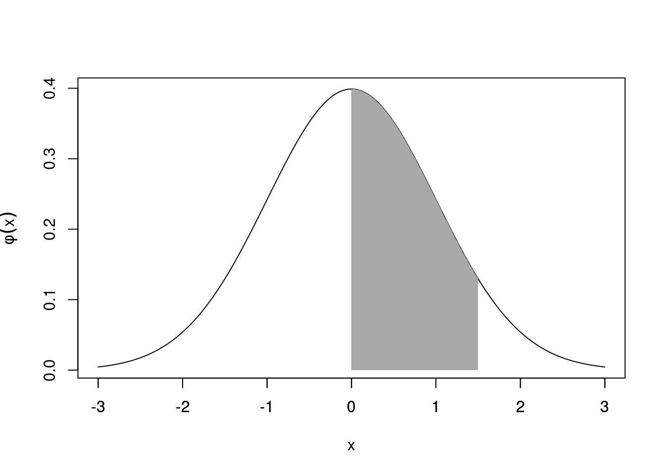
Figure 21.8: \(P(0<X<x)\) is the area under \(\phi(x)\) from \(0\) to \(x\)
| 0 | 0.01 | 0.02 | 0.03 | 0.04 | 0.05 | 0.06 | 0.07 | 0.08 | 0.09 | |
|---|---|---|---|---|---|---|---|---|---|---|
| 0 | 0.0000 | 0.0040 | 0.0080 | 0.0120 | 0.0160 | 0.0199 | 0.0239 | 0.0279 | 0.0319 | 0.0359 |
| 0.1 | 0.0398 | 0.0438 | 0.0478 | 0.0517 | 0.0557 | 0.0596 | 0.0636 | 0.0675 | 0.0714 | 0.0753 |
| 0.2 | 0.0793 | 0.0832 | 0.0871 | 0.0910 | 0.0948 | 0.0987 | 0.1026 | 0.1064 | 0.1103 | 0.1141 |
| 0.3 | 0.1179 | 0.1217 | 0.1255 | 0.1293 | 0.1331 | 0.1368 | 0.1406 | 0.1443 | 0.1480 | 0.1517 |
| 0.4 | 0.1554 | 0.1591 | 0.1628 | 0.1664 | 0.1700 | 0.1736 | 0.1772 | 0.1808 | 0.1844 | 0.1879 |
| 0.5 | 0.1915 | 0.1950 | 0.1985 | 0.2019 | 0.2054 | 0.2088 | 0.2123 | 0.2157 | 0.2190 | 0.2224 |
| 0.6 | 0.2257 | 0.2291 | 0.2324 | 0.2357 | 0.2389 | 0.2422 | 0.2454 | 0.2486 | 0.2517 | 0.2549 |
| 0.7 | 0.2580 | 0.2611 | 0.2642 | 0.2673 | 0.2704 | 0.2734 | 0.2764 | 0.2794 | 0.2823 | 0.2852 |
| 0.8 | 0.2881 | 0.2910 | 0.2939 | 0.2967 | 0.2995 | 0.3023 | 0.3051 | 0.3078 | 0.3106 | 0.3133 |
| 0.9 | 0.3159 | 0.3186 | 0.3212 | 0.3238 | 0.3264 | 0.3289 | 0.3315 | 0.3340 | 0.3365 | 0.3389 |
| 1 | 0.3413 | 0.3438 | 0.3461 | 0.3485 | 0.3508 | 0.3531 | 0.3554 | 0.3577 | 0.3599 | 0.3621 |
| 1.1 | 0.3643 | 0.3665 | 0.3686 | 0.3708 | 0.3729 | 0.3749 | 0.3770 | 0.3790 | 0.3810 | 0.3830 |
| 1.2 | 0.3849 | 0.3869 | 0.3888 | 0.3907 | 0.3925 | 0.3944 | 0.3962 | 0.3980 | 0.3997 | 0.4015 |
| 1.3 | 0.4032 | 0.4049 | 0.4066 | 0.4082 | 0.4099 | 0.4115 | 0.4131 | 0.4147 | 0.4162 | 0.4177 |
| 1.4 | 0.4192 | 0.4207 | 0.4222 | 0.4236 | 0.4251 | 0.4265 | 0.4279 | 0.4292 | 0.4306 | 0.4319 |
| 1.5 | 0.4332 | 0.4345 | 0.4357 | 0.4370 | 0.4382 | 0.4394 | 0.4406 | 0.4418 | 0.4429 | 0.4441 |
| 1.6 | 0.4452 | 0.4463 | 0.4474 | 0.4484 | 0.4495 | 0.4505 | 0.4515 | 0.4525 | 0.4535 | 0.4545 |
| 1.7 | 0.4554 | 0.4564 | 0.4573 | 0.4582 | 0.4591 | 0.4599 | 0.4608 | 0.4616 | 0.4625 | 0.4633 |
| 1.8 | 0.4641 | 0.4649 | 0.4656 | 0.4664 | 0.4671 | 0.4678 | 0.4686 | 0.4693 | 0.4699 | 0.4706 |
| 1.9 | 0.4713 | 0.4719 | 0.4726 | 0.4732 | 0.4738 | 0.4744 | 0.4750 | 0.4756 | 0.4761 | 0.4767 |
| 2 | 0.4772 | 0.4778 | 0.4783 | 0.4788 | 0.4793 | 0.4798 | 0.4803 | 0.4808 | 0.4812 | 0.4817 |
| 2.1 | 0.4821 | 0.4826 | 0.4830 | 0.4834 | 0.4838 | 0.4842 | 0.4846 | 0.4850 | 0.4854 | 0.4857 |
| 2.2 | 0.4861 | 0.4864 | 0.4868 | 0.4871 | 0.4875 | 0.4878 | 0.4881 | 0.4884 | 0.4887 | 0.4890 |
| 2.3 | 0.4893 | 0.4896 | 0.4898 | 0.4901 | 0.4904 | 0.4906 | 0.4909 | 0.4911 | 0.4913 | 0.4916 |
| 2.4 | 0.4918 | 0.4920 | 0.4922 | 0.4925 | 0.4927 | 0.4929 | 0.4931 | 0.4932 | 0.4934 | 0.4936 |
| 2.5 | 0.4938 | 0.4940 | 0.4941 | 0.4943 | 0.4945 | 0.4946 | 0.4948 | 0.4949 | 0.4951 | 0.4952 |
| 2.6 | 0.4953 | 0.4955 | 0.4956 | 0.4957 | 0.4959 | 0.4960 | 0.4961 | 0.4962 | 0.4963 | 0.4964 |
| 2.7 | 0.4965 | 0.4966 | 0.4967 | 0.4968 | 0.4969 | 0.4970 | 0.4971 | 0.4972 | 0.4973 | 0.4974 |
| 2.8 | 0.4974 | 0.4975 | 0.4976 | 0.4977 | 0.4977 | 0.4978 | 0.4979 | 0.4979 | 0.4980 | 0.4981 |
| 2.9 | 0.4981 | 0.4982 | 0.4982 | 0.4983 | 0.4984 | 0.4984 | 0.4985 | 0.4985 | 0.4986 | 0.4986 |
| 3 | 0.4987 | 0.4987 | 0.4987 | 0.4988 | 0.4988 | 0.4989 | 0.4989 | 0.4989 | 0.4990 | 0.4990 |
Example 21.3 (Using Statistical Tables) What is \(P(-0.45<X<1.25)\) for a standard normal variable \(X\)?
Using table 21.1 \[\begin{eqnarray*} P(-0.45<X<1.25) &=&P(X<1.25)\\ && \quad - P(X<-0.45)\\ &=&P(X<1.25)\\ && \quad -\left[1 - P(X<0.45)\right]\\ &\approx&0.8944-(1 - 0.6736)\\ &\approx&0.568 \end{eqnarray*}\]
Or using table 21.2 \[\begin{eqnarray*} P(-0.45<X<1.25) &=&P(0<X<1.25)\\ && \quad + P(0<X<0.45)\\ &=&0.3944+0.1736\\ &\approx&0.568 \end{eqnarray*}\]
We can use standard tables to find probabilities of general normal random variables. If \(Y\) is normal with mean \(\mu\) and variance \(\sigma^2\), then \[X=(Y-\mu)/\sigma\] is standard normal. Then for \(a<b\), \[\begin{eqnarray*} P(a\le Y\le b)&=&P(a\le \sigma X+\mu\le b)\\ &=&P\left(\frac{a-\mu}\sigma\le X\le\frac{b-\mu}\sigma\right)\\ &=&\Phi\left(\frac{b-\mu}\sigma\right)-\Phi\left(\frac{a-\mu}\sigma\right). \end{eqnarray*}\]
Example 21.4 (Non-standard normal random variables)
If \(Y\) is normal with mean \(1\) and variance \(4=2^2\), then \(X=(Y-1)/2\) is . Calculate \(P(0<Y<2.5)\).
Using table 21.1 \[\begin{eqnarray*} P(0<Y<2.5)&=&P(-0.5<X<0.75)\\ &=&P(X<0.75)-\left[1 - P(X<0.5)\right]\\ &\approx&0.7734 - (1 - 0.6915)\approx 0.4649 \end{eqnarray*}\]
or using table 21.2 \[\begin{eqnarray*} P(0<Y<2.5)&=&P(-0.5<X<0.75)\\ &=&P(0<X<0.75)+ P(0<X<0.5)\\ &\approx&0.2734 + 0.1915\approx 0.4649 \end{eqnarray*}\]
If \(Y\) is normal with mean \(3\) and variance \(25\), calculate \(P(4<Y<8)\).
\[\begin{eqnarray*} P(4<Y<8)&=&P(0.2<X<1)\\ &=&P(X<1)- P(X<0.2)\\ &\approx 0.8413 - 0.5793 & \approx 0.262. \end{eqnarray*}\]
or
\[\begin{eqnarray*} P(4<Y<8)&=&P(0.2<X<1)\\ &=&P(0<X<1)-P(0<X<0.2)\\ &\approx&0.3413 - 0.0793\approx 0.262. \end{eqnarray*}\]
If \(X\) is standard normal, we find \[\begin{eqnarray*} P(|X|>2)&=&1-P(-2<X<2)\\ &=&2 P(X > 2)\\ &=&2 \left[1 - P(X < 2)\right]\\ &\approx& 2 \times (1 - 0.9772)\\ &=& 0.0456. \end{eqnarray*}\]
Hence approx. 95% of the distribution lies in the region \(-2 < X < 2\) (or in the case of a general normal random variable \(Y\) this region is between \(\mu\pm2\sigma\)).
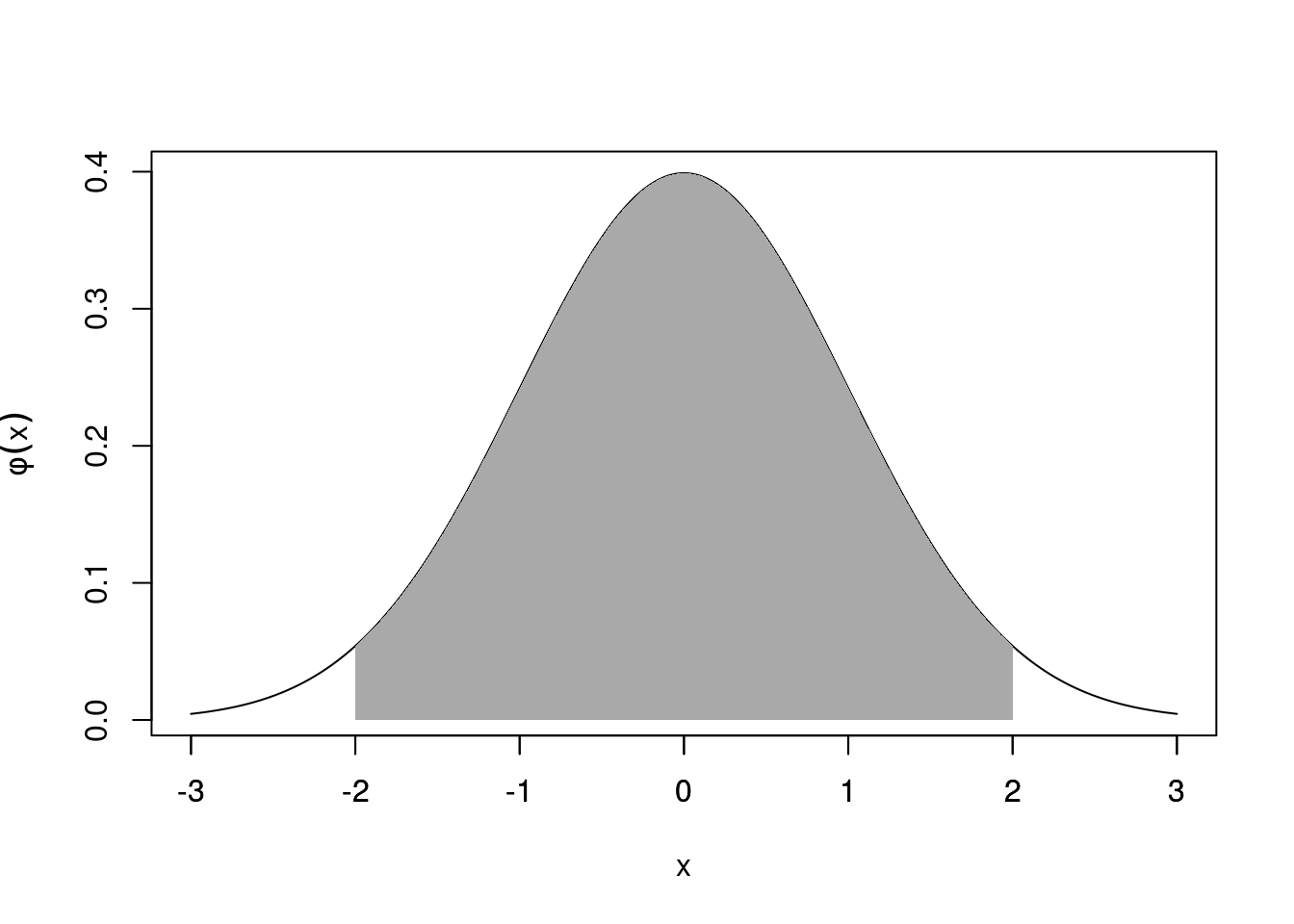
Figure 21.9: Approximately 95% lies within \(\pm2\sigma\).
Linear interpolation
Note that if the exact value you are looking for isn’t tabulated then one option would be to round to the nearest value. A more accurate approximation is to use linear interpolation between the two nearest values given in the table e.g. you want \(\Phi(c)\) and nearest values in table are \(\Phi(a)\) and \(\Phi(b)\) where \(a < c < b\), then approximate \[ \Phi(c) = \Phi(a) + \left(\frac{c - a}{b - a}\right)(\Phi(b) - \Phi(a)). \] (Make sure you adjust appropriately if finding \(1 - \Phi(c)\).)
21.6 The Law of Large Numbers
The concept of the “law of averages” can be made mathematically respectable and precise through a result known as the law of large numbers.
Suppose \(X_1, \dots, X_n\) is a sequence of independent identically distributed (i.i.d.) random variables such that \(E(X_i) = \mu\) and \(\operatorname{var}(X_i) = \sigma^2\) for \(i = 1, \dots, n\), and let \[ \bar{X} = \frac{1}{n} \sum_{i=1}^n X_i \] denote the sample mean (so-called because one can think of the sequence \(X_1, \dots, X_n\) as conceptually representing repeated independent samples (observations) from the same probability distribution).
The law of large numbers then states that the probability that the difference between \(\bar{X}\) and \(\mu\) is arbitrarily small can be made close to 1 by taking a large enough sample.
21.7 Central Limit Theorem
The reason the normal distribution is so ubiqitous is due to the Central Limit Theorem (CLT).
Informally, the CLT states that the average of a set of i.i.d. random variables each of which has mean \(\mu\) and variance \(\sigma^2\) is approximately normally distributed with mean \(\mu\) and variance \(\frac{\sigma^2}{n}\) if \(n\) is large.
Hence, if \(\bar{X} = \frac{1}{n} \sum_{i = 1}^n X_i\), then \(\bar{X} \sim N\left(\mu, \frac{\sigma^2}{n}\right)\) for large \(n\) whatever distribution the \(X_i\) have.
Example 21.5 (Central Limit Theorem) You repeatedly throw a fair die \(n\) times and take the average of the scores.
Here, \(X_i\) is the score on the \(i^{\text{th}}\) die, and \(\displaystyle{\bar{X} = \frac{1}{n} \sum_{i=1}^n X_i}\) is the mean score, then \(\bar{X}\) will approximately follow a \(N\left(3.5, \frac{2.92}{n}\right)\) distribution for large \(n\).
Another way of stating the CLT is that as \(n \to \infty\) the probability distribution of \(\left(\frac{X - \mu}{\sigma / \sqrt{n}}\right)\) tends to a standard normal distribution.
What is remarkable about this theorem is that it applies whatever probability distribution \(X_i\) has. It can be discrete or continuous, and of any type, Binomial, Poisson, uniform, normal,…