Chapter 11 Differentiation

11.1 Concept

Differentiation is the mathematical tool to answer questions about rates of change.

The derivative of a real function $f$ at a point $(x,f(x))$ is the slope of the tangent line at that point.

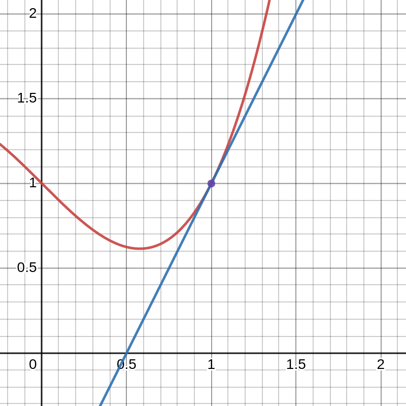
Figure 11.1: The tangent line to a graph.

To find this gradient, we start by approximating the tangent line by taking a secant line through the point $(x,f(x))$ and a point $(x+h,f(x+h))$ with $h$ a small number.

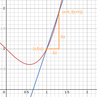
Figure 11.2: A secant line through $(x,f(x))$ and a point $(x+h,f(x+h))$.

Now if we take $h\to 0$, that is $h$ becomes vanishingly small, the second point approaches $(x,f(x))$. Then the gradient of the secant line converges to the gradient of the tangent line. The gradient of the secant line is: \[ \frac{\Delta y}{\Delta x}=\frac{f(x+h)-f(x)}{h}. \]

The mathematical term for taking $h\to 0$ is taking the limit as $h$ tends to $0$, written

\[ \lim\limits_{h\to 0}\frac{f(x+h)-f(x)}{h}. \]

The idea here is to consider what happens to this mathematical expression as $h$ becomes infinitesimally small. We call this gradient of the tangent line the derivative of $f$ at $x$. We use the following notations for the derivative:

\[f'(x)\quad\text{ or }\quad \frac{df}{dx} \]

Here we present some examples of finding derivatives from first principles, i.e. by using the limit definition of the derivative.

Example 11.1 (Derivatives from first principles) The first two examples are applied to straight lines, whose tangents are the same as the lines themselves, hence we should get the same gradient from the derivative.

Consider a constant function $f(x)=c$ (the graph of which is a straight horizontal line). We know that the gradient of this line is zero. Let’s try applying the definition. \[\begin{align*} f'(x)&=\lim\limits_{h\to 0}\frac{f(x+h)-f(x)}{h}\\ &=\lim\limits_{h\to 0}\frac{c-c}{h}\quad\text{applying the definition of $f$}\\ &=\lim\limits_{h\to 0}\frac{0}{h}\\ &=\lim\limits_{h\to 0}0\quad\text{note this expression is now independent of the value of $h$, hence...}\\ &=0 \end{align*}\] in agreement with our geometical understanding.
Consider a straight line of the form $f(x)=mx+c$. Using the definition of the derivative \[\begin{align*} f'(x)&=\lim\limits_{h\to 0}\frac{f(x+h)-f(x)}{h}\\ &=\lim\limits_{h\to 0}\frac{[m(x+h)+c]-[mx+c]}{h}\quad\text{applying the definition of $f$}\\ &=\lim\limits_{h\to 0}\frac{mh}{h}\\ &=\lim\limits_{h\to 0}m\quad\text{note this expression is now independent of the value of $h$, hence...}\\ &=m. \end{align*}\] again in agreement with our geometical understanding.
Consider $f(x)=x^2$. \[\begin{align*} f'(x)&=\lim\limits_{h\to 0}\frac{f(x+h)-f(x)}{h}\\ &=\lim\limits_{h\to 0}\frac{(x+h)^2-x^2}{h}\quad\text{applying the definition of $f$}\\ &=\lim\limits_{h\to 0}\frac{x^2+2xh+h^2-x^2}{h}\quad\text{expanding brackets}\\ &=\lim\limits_{h\to 0}2x+h\quad\text{by simplifying}\\ &=2x\quad\text{since $h$ becomes vanishingly small.} \end{align*}\]

It would be hard work if we always had to apply the definition to find the derivatives of functions. Thankfully, others have already done the hard work and we have some rules for derivatives of standard functions, together with some rules for derivatives of combinations of functions (including sums, products and compositions). This allows us to compute the derivatives of a wide variety of expressions we might encounter.

11.2 Standard derivatives

\[\begin{align*} &\frac{d}{dx}x^a=ax^{a-1}\qquad \text{for any $a\in\mathbb{R}$}\\ &\\ &\frac{d}{dx}\ln(x)=\frac{1}{x}\\ &\frac{d}{dx}e^{x}=e^{x}\\ &\\ &\frac{d}{dx}\sin(x)=\cos(x)\\ &\frac{d}{dx}\cos(x)=-\sin(x)\\ &\frac{d}{dx}\tan(x)=\sec^2(x)\\ &\\ &\frac{d}{dx}\sinh(x)=\cosh(x)\\ &\frac{d}{dx}\cosh(x)=\sinh(x) \end{align*}\]

11.3 Rules

Sum Rule

\[ (f+g)'(x)=f'(x)+g'(x) \]

Example 11.2 Find the derivative of \[h(x)=x^3+\sin(x).\] Let $f(x)=x^3$, $g(x)=\sin(x)$. Then \[h(x)=(f+g)(x)=x^3+\sin(x)\] and \[h'(x)=(f+g)'(x)=f'(x)+g'(x)=3x^2+\cos(x).\]

Product Rule

\[ (f\cdot g)'(x)=f'(x)\cdot g(x)+f(x)\cdot g'(x) \]

Example 11.3 Find the derivative of \[h(x)=x^3\sin(x)\] Let $f(x)=x^3$, $g(x)=\sin(x)$. Then \[h(x)=(f\cdot g)(x)=x^3\sin(x)\] and \[h'(x)=(f\cdot g)'(x)=f'(x)g(x)+f(x)g'(x)=3x^2\sin(x)+x^3\cos(x).\]

In particular (exercise), for any constant $a$ we have: $(af(x))'=af'(x)$.

Quotient Rule

\[ \left(\dfrac{f}{g}\right)'(x)=\frac{g(x)\cdot f'(x)-f(x)\cdot g'(x)}{[g(x)]^2} \]

Example 11.4 Find the derivative of \[h(x)=\frac{x^3}{\sin(x)}.\] Let $f(x)=x^3$, $g(x)=\sin(x)$. Then \[h(x)=(\frac{f}{g})(x)=\frac{x^3}{\sin(x)}\] and \[h'(x)=(\frac{f}{g})'(x)=\frac{g(x)\cdot f'(x)-f(x)\cdot g'(x)}{[g(x)]^2}=\frac{3x^2\sin(x)-x^3\cos(x)}{\sin^2(x)}.\]

Chain Rule

\[ \left(f\circ g\right)'(x)=f'(g(x))\cdot g'(x) \]

(where $\left(f\circ g\right)(x)=f(g(x))$ denotes function composition).

Example 11.5 Find the derivative of \[h(x)=\sin(x^3)\] Let $f(x)=\sin(x)$, $g(x)=x^3$. Then \[h(x)=(f\circ g)(x)=\sin(x^3)\] and \[h'(x)=(f\circ g)'(x)=f'(g(x))\cdot g'(x)=\cos(x^3)(3x^2)=3x^2\cos(x^3).\]

The key to using these rules is in splitting your function $h(x)$ into the right combination of two or more simpler functions ($f(x)$ and $g(x)$ in the above examples) to make it easy to apply the rules.

11.4 Higher order derivatives

The derivative of a function $f$ is also a function, which we denote $f'$. We can also take the derivative of the function $f'$, yielding the function $(f')'$, which is usually written as $f''$, and is called the second derivative of $f$. For example, with $f(x)=x^3$ we have $f'(x)=3x^2$ and $f''(x)=6x$.

There is no reason to stop at the second derivative, and we can define $f'''=(f'')'$, $f''''=(f''')'$ etc. After a few derivatives of $f$ it is more convenient to use the notation: \[\begin{align*} f^{(0)}&=f\\ f^{(1)}&=f'\\ f^{(2)}&=(f')'=f''\\ f^{(3)}&=(f'')'=f'''\\ &\phantom{..}\vdots\\ f^{(n+1)}&=(f^{(n)})' \end{align*}\] The functions $f^{(n)}$ for $n\geq 2$ are called higher-order derivatives.

Derivatives may also be denoted using Leibniz notation: \[ \frac{df(x)}{dx} \] This notation ties in with Leibniz’s intuitive notion of the derivative as the quotient of the “infinitely small difference $df(x)=f(x+dx)-f(x)$”, by the “infinitely small number $dx$”; but it is important to note that the derivative is defined as the limit, and the symbols $df(x)$ and $dx$ have no meaning of their own, and cannot be manipulated separately.

Higher order derivatives are denoted \[ \frac{d^2f(x)}{dx^2},\frac{d^3f(x)}{dx^3},\dotsc,\frac{d^nf(x)}{dx^n},\dotsc \]

Leibniz’s Formula allows us to easily compute higher order derivatives of products.

The $n^\text{th}$ derivative of the product $(f\cdot g)(x)$ is \[ (f\cdot g)^{(n)}(x)=\sum_{k=0}^{n}\binom{n}{k}f^{(k)}(x)\cdot g^{(n-k)}(x). \]

Recall that the binomial coefficient is given by: \[ \binom{n}{k}=\frac{n!}{k!(n-k)!}. \]

11.5 Further Techniques

11.5.1 Implicit Differentiation

Curves in the plane are often described by the set of all coordinates $(x,y)$ satisfying an equation of the form ${F(x,y)=0}$ for some function $F$ of two variables.

For example, the unit circle is described by the equation $F(x,y)=x^2+y^2-1=0$.

As with the circle, we often cannot describe such a curve in the form of a graph of a function $y=f(x)$ (since it is multivalued for each $x$). How do we differentiate such a curve?

Example 11.6

The unit circle $x^2+y^2=1$ has a well defined slope at every point except $(-1,0)$ and $(1,0)$ where there are vertical tangents. For the circle we can quite easily find functions that describe the differentiable parts of the curve: \[\begin{align*} f_1(x)&=\sqrt{1-x^2} &-1< x < 1\\ f_2(x)&=-\sqrt{1-x^2} &-1< x < 1 \end{align*}\] which describe the upper and lower halves of the circle, respectively.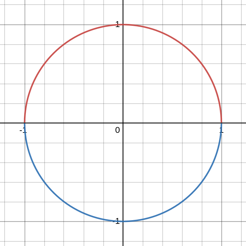

Figure 11.3: Functions describing the upper an lower parts of the circle

Then to obtain the derivative at any point on the circle (except $(-1,0),(1,0)$), we can calculate the derivative of the relevant function $f_1$ or $f_2$: \[ f_1'(x)=\dfrac{-x}{(1-x^2)^\frac{1}{2}},\qquad f_2'(x)=\dfrac{x}{(1-x^2)^\frac{1}{2}}. \]

For the circle we are able to write down differentiable functions with explicit formulae. In general, however, it will not be possible, or at least not easy, to find such functions.

A function $f$ defined by the fact that it satisfies an equation $F(x,f(x))=0$ is called an implicit function; it is defined implicitly, rather than by an explicit formula.

In general, the coordinates where $F(x,y)=0$ may not be describable by the graph of a differentiable function. Even where it is, there may be more than one function defined by the relation, as was the case with the circle. Furthermore, it may not be possible to write down $f$ as a nice formula as we did for the circle.

If we assume that a function $f$ is a differentiable solution to the equation, then we can derive a formula for $f'$ by the process of implicit differentiation. (We will only deal with simple cases here anyway and so need not be concerned with the technichal details, but in general we would need to turn to the Implicit Function Theorem to guarantee that all technichal assumptions are valid.)

The process has two main steps:

Differentiate both sides of the equation with respect to $x$, treating $y$ as a differentiable function of $y(x)$ and using the Chain Rule.
Solve for $y'(x)$, giving a formula involving $x$ and $y$ that yields the derivative at any point $(x,y)$ on the curve $F(x,y)=0$.

Example 11.7 (Implicit differentiation) Consider the unit circle $x^2+y^2=1$. We treat $y=y(x)$ as a differentiable function. \[\begin{align*} \frac{d}{dx}(x^2+y^2)&=\frac{d}{dx}(1)\\ \frac{d}{dx}(x^2)+\frac{d}{dx}(y^2)&=0\\ 2x+2y\frac{dy}{dx}&=0\\ \frac{dy}{dx}&=-\frac{x}{y} \end{align*}\] Where in the third line we have used the chain rule, by setting $y=y(x)$ so that \[ \frac{d}{dx}(y(x)^2)=2y(x)\dfrac{d}{dx}(y(x)). \] Note that we have “infinite gradients” if $y=0$, as we had already stated.

Note that this agrees with our previous analysis: if $(a,b)$ lies on the upper half of the circle then the slope at this point is given by \[ f_1'(a)=\dfrac{-a}{(1-a^2)^\frac{1}{2}} \] or using the above implicit derivative and the formula for $f_1$ \[ \frac{dy}{dx}=-\frac{a}{b}=-\frac{a}{f_1(a)}=-\frac{a}{\sqrt{1-a^2}}. \] and similarly for a point on the lower half of the circle.

11.5.2 Logarithmic Differentiation

By the chain rule, the derivative of $\ln\circ f$ is $\dfrac{f'}{f}$, and this will often be easier to compute than $f'$ because logarithms turn products into sums, and powers into products. The derivative for $f$ can then be recovered by multiplying through by $f$.

This process is known as logarithmic differentiation.

Example 11.8 (Logarithmic differentiation) Find the derivative of \[ y=x^x. \] First take the natural logarithm: \[ \ln(y)=x\ln(x), \] then differentiate implicitly: \[\begin{align*} \frac{d}{dx}(\ln(y))&=\frac{d}{dx}(x\ln(x))\\ \frac{1}{y}\frac{dy}{dx}&=\frac{dx}{dx}\ln(x)+x\frac{d}{dx}\ln(x)\\ \frac{1}{y}\frac{dy}{dx}&=\ln(x)+x\frac{1}{x}\\ \frac{dy}{dx}&=y(\ln(x)+1)=x^x(\ln(x)+1). \end{align*}\]

Warning! The derivative of $x^x$ is $x\cdot x^{x-1}$. We can’t treat variable exponents like constant exponents!

11.5.3 Parametric Differentiation

Curves in the plane may also be described parametrically. Given two functions $u(t)$ and $v(t)$, the curve \[ \{(x,y): x=u(t), y=v(t)\} \] is said to be represented parametrically by $u$ and $v$, and the pair of functions $u$ and $v$ are called a parametric representation of the curve.

We can think of such a curve as being the path traced out by a particle moving in the plane; at time $t$ the particle is at the position with coordinates $(u(t),v(t))$. A parametric curve is a function from the real numbers into the plane, given by $F(t)=(u(t),y(t))$. Such curves will generally not be the graph of a function (due to being multivalued for a given $x$-coordinate).

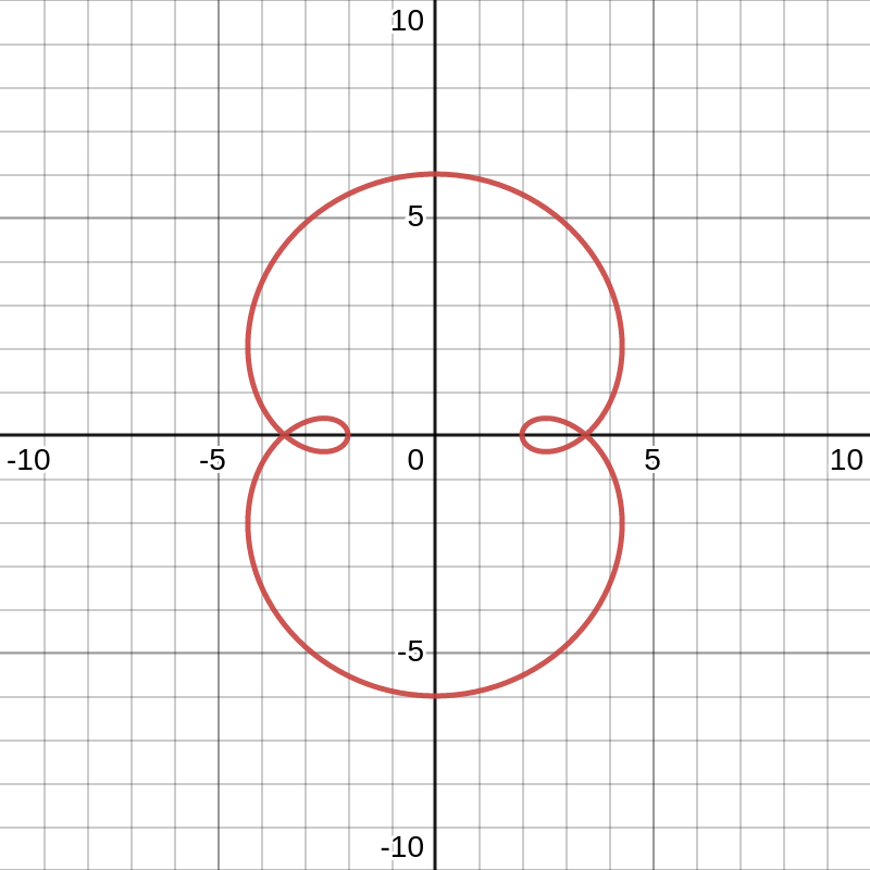
$The parametric curve given by $x(\theta)=4\sin(\theta)+2\sin(3\theta)$ and $y(\theta)=4\cos(\theta)+2\cos(3\theta)$.$

Figure 11.4: The parametric curve given by $x(\theta)=4\sin(\theta)+2\sin(3\theta)$ and $y(\theta)=4\cos(\theta)+2\cos(3\theta)$.

How do we differentiate such a curve?

Suppose that ${x=u(t)}$, ${y=v(t)}$ is a parametric representation of a curve, and that $u'\neq 0$ on some interval. Then on this interval the curve lies on the graph of a function $f$, and at the point $x=u(t)$ \[ f'(x)=\frac{v'(t)}{u'(t)} \]

To see this, we have ${v(t)=f(x(t))}$, so differentiating with respect to $t$ and using the chain rule on the right hand side, \[ v'(t)=f'(x)u'(t) \] and since $u'(t)\neq 0$ \[ f'(x)=\frac{v'(t)}{u'(t)}. \]

In Leibniz notation this is often written as: \[ \frac{dy}{dx}=\frac{\dfrac{dy}{dt}}{\dfrac{dx}{dt}} \] and one can imagine “cancelling the $dt$’s”.

Example 11.9 (Parametric differentiation) An ellipse $\dfrac{x^2}{a^2}+\dfrac{y^2}{b^2}=1$ can be represented parametrically by ${x=a\cos(\theta), y=b\sin(\theta)}$. The derivative at a point on the ellipse corresponding to parameter value $\theta$ is: \[\begin{align*} \frac{dy}{dx}&=\frac{dy/d\theta}{dx/d\theta}\\ &=-\frac{b\cos(\theta)}{a\sin(\theta)}\\ &=-\frac{b}{a}\cot(\theta). \end{align*}\]

Second order parametric derivatives. Suppose that $x=u(t)$, $y=v(t)$, then \[ \frac{d^2y}{dx^2}=\frac{d}{dx}\left(\frac{dy}{dx}\right)=\frac{d}{dx}\left(\frac{\dfrac{dy}{dt}}{\dfrac{dx}{dt}}\right) \] and we can compute this using the chain rule: \[ \frac{d^2y}{dx^2}=\frac{d}{dt}\left(\frac{dy}{dx}\right)\frac{dt}{dx}. \] Alternatively, we could use the quotient rule, but this is more complicated: \[ \frac{d^2y}{dx^2}=\frac{\frac{dx}{dt}\frac{d^2y}{dt^2}-\frac{dy}{dt}\frac{d^2x}{dt^2}}{\left( \frac{dx}{dt}\right)^3}. \]