Chapter 2 Functions and Graphs
A function \(f\) can be thought of as a machine that takes an input value \(x\) and returns an output value \(y\). The output value \(y\) corresponding to the input \(x\) is also denoted by \(f(x)\) (read “\(f\) of \(x\)”). We most commonly encounter functions whose input is a real number and output is a real number, but there are many other types of functions in mathematics.
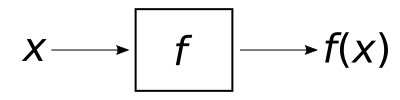
Figure 2.1: A function can be thought of as a machine: we have an input value \(x\), the machine is the function \(f\), and the output is the value \(f(x)\)
We are familiar with plotting such functions on a graph, where we draw the coordinates \((x,f(x))\), or \((x,y)\), against perpendicular axes – this is known as the Cartesian coordinate system.
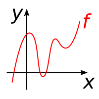
Figure 2.2: A function can be plotted in Cartesian Coordinates: the corresponding inputs \(x\) and outputs \(y=f(x)\) are plotted as a point; these often form a continuous curve in the plane.
In this section we shall take a look at some useful functions, their graphs, and some of their other interesting properties.
2.1 Linear Functions
We are familiar with the equation of a straight line: \[y=mx+d\] with gradient \(m\) and intercepting the \(y\)-axis at the value \(d\).
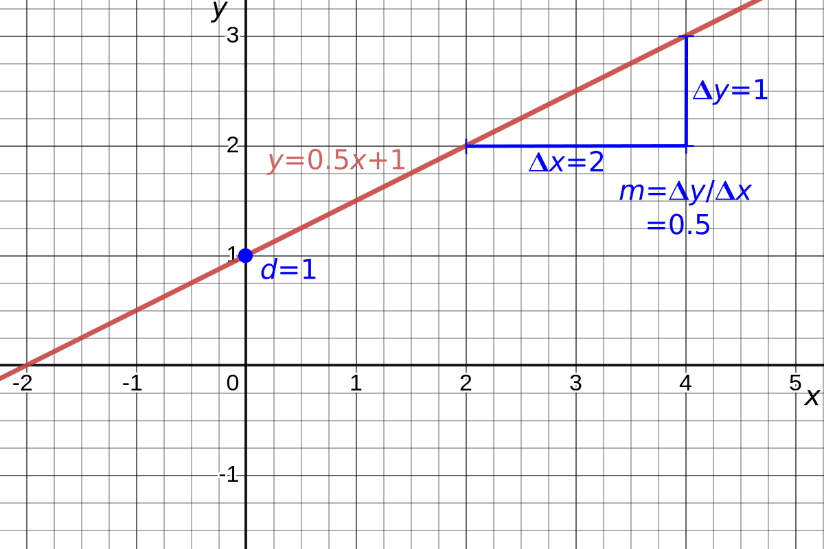
Figure 2.3: Straight line graph of \(y=\frac{1}{2}x+1\).
If we think about such a line as a function with input \(x\) and output \(y\), then we call this a linear function.
If the gradient is positive, \(m>0\), then the line slopes upwards with increasing \(x\) values; if the gradient is negative, \(m<0\), then the line slopes downwards with increasing \(x\) values; if the gradient is zero, \(m=0\), then the line is a horizontal line. Note that we cannot describe a vertical line with this function: a vertical line has an equation of the form \(x=A\), where \(A\) is the value at which it intercepts the \(x\)-axis.
Specifying a single point \((x_1,y_1)\) and a gradient \(m\) is enough to define a (non-vertical) line and we can write the equation of this line as \[ y-y_1=m(x-x_1). \]
Also, a line can be defined by specifying any two points \((x_1,y_1)\) and \((x_2,y_2)\) that lie on the line. We can calculate the gradient of this line from \[ m=\frac{y_2-y_1}{x_2-x_1} \] but there is a problem if \(x_2=x_1\) and we have division by \(0\) – effectively we have an “infinite” gradient. Since \(x_1=x_2\) this, of course, corresponds to a vertical line, which we can write as the equation \(x=x_1\).
An equation of the form \(ax+by+c=0\) is a general way to express any line in the Cartesian plane and includes both vertical and non-vertical lines. In section ?? we will be using this more general form for solving simultaneous linear equations.
Figure 2.4: A general line \(ax+by+c=0\) (red line) a line specified by a gradient and intercept \(y=mx+d\) (blue line), a vertical line \(x=A\) (green line) and a horizontal line \(y=B\) (orange line). Adjust the sliders to change the constants and check which values of \(m,d,A,\) and \(B\) correspond to \(a,b\) and \(c\). [Open graph in browser.]
2.1.1 Parallel lines
A line makes an angle \(\theta\) from the positive \(x\)-axis, the angle of inclination. This is related to the gradient \(m\) by \[ m=\frac{\Delta y}{\Delta x}=\tan(\theta). \] Two lines are parallel if they have the same angle of inclination \(\theta\), or same gradient \(m\).
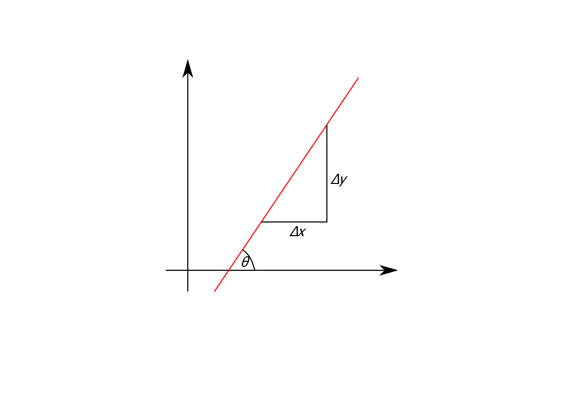
Figure 2.5: The angle of inclination of a line.
Hence if two (non-vertical) lines are parallel they are of the form \[\begin{align*} y&=mx + d_1\\ y&=mx + d_2 \end{align*}\] with different \(y\)-intercepts \(d_1\) and \(d_2\).
2.1.2 Perpendicular lines
Two lines are perpendicular, or normal, if they meet at a right angle. We have \[\begin{align*} m_1&=\tan(\theta)\quad\text{and,}\\ m_2&=\tan\Big(\theta + \frac{\pi}{2}\Big)=\frac{\sin(\theta + \frac{\pi}{2})}{\cos(\theta + \frac{\pi}{2})}\\ &=\frac{\sin(\theta)\cos(\frac{\pi}{2}) + \cos(\theta)\sin(\frac{\pi}{2})}{\cos(\theta)\cos(\frac{\pi}{2}) - \sin(\theta)\sin(\frac{\pi}{2})}\\ &=\frac{\cos(\theta)}{-\sin(\theta)}\\ &=-\cot(\theta) \end{align*}\]
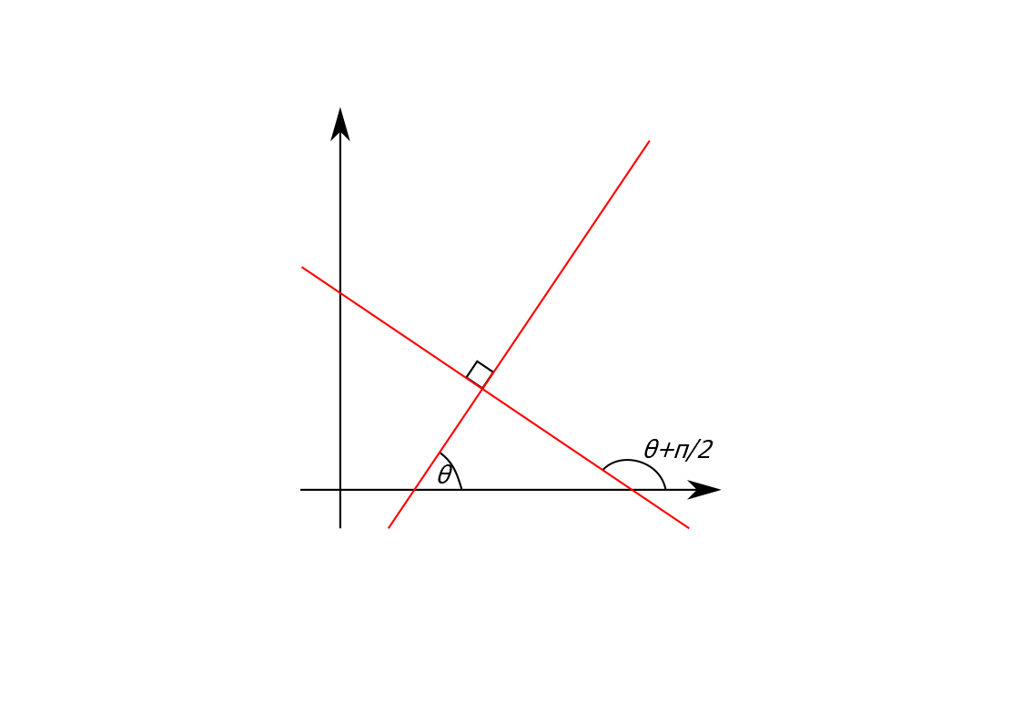
Figure 2.6: Perpendicular lines.
Thus, two (non-vertical) lines are perpendicular if \[\begin{equation*} m_1m_2=-1 \end{equation*}\] and hence they have the forms \[\begin{align*} y&=mx + d_1,\\ y&=-\frac{1}{m}x + d_2. \end{align*}\] with \(y\)-intercepts \(d_1\) and \(d_2\).
Alternatively, if we describe a line by \(ax+by+c=0\) then \[\begin{align*} ax+by+p&=0\quad\text{is a parallel line}\\ bx+ay+q&=0\quad\text{is a perpendicular line} \end{align*}\] where \(p\) and \(q\) are constants.
2.2 Polynomials
A polynomial is a function made up of non-negative integer powers of the independent variable \(x\) multiplied by constant coefficients, i.e. it has the form
\[f(x)=a_0 + a_1 x + a_2 x^2 + \dotsb + a_n x^n\]
where the \(n+1\) fixed numbers \(a_0,\dots,a_n\) are the coefficients (which could be positive, negative or zero). For example, the following are all polynomials: \[\begin{align*} f(x)&=x^2\\ g(x)&=2+\frac{1}{3}x^4 - x^5\\ h(x)&=-3.6 + x^2 -2x^{10} \end{align*}\]
The number \(n\) corresponding to the highest power in the polynomial is called the order or degree of the polynomial. For the functions \(f, g\) and \(h\) above the degrees are \(2, 5\) and \(10\), respectively. We have a few special names for polynomials of low degree:
- Degree 1: a linear polynomial, since its graph is a line \(f(x)=a_0+a_1 x\)
- Degree 2: a quadratic polynomial
- Degree 3: a cubic polynomial
- Degree 4: a quartic polynomial
- Degree 5: a quintic polynomial
The higher the degree of the polynomial, the more “wavey” its graph can be; in fact, a degree \(n\) polynomial can have at most \(n-1\) turning points.
A polynomial which has only one term is called a monomial, for example
\[f(x)=2\\ g(x)=3x^2\\ h(x)=-4x^5 \]
are all monomials.
Figure 2.7: A plot of a polynomial of at most degree 5, \(f(x)=a_0 + a_1 x + a_2 x^2 + a_3 x^3 + a_4 x^4 + a_5 x^5\). Adjust the sliders to change the coefficients \(a_0\) to \(a_5\) to get a feel for the possible shapes of a degree 5 polynomial; set the higher degree coefficients to \(0\) to look at lower degree polynomials; also take a look at the monomials up to degree 5. [Open graph in browser.]
2.3 Rational functions
A rational function is one that can be expressed as the quotient of two polynomials, for example
\[f(x)=\frac{1+x}{2-x+3x^2}\]
is the quotient of a degree 1 polynomial and a degree 2 polynomial.
They often have values of \(x\) where they are undefined due to the denominator evaluating to zero. Furthermore, they often have asymptotes, which means the graph approaches a straight line.
For example, the function \(f(x)=\frac{x^{2}}{x^{2}-4}\) has asmptotes at the vertical lines \(x=2\) and \(x=-2\) and at the horizontal line \(y=1\).
Figure 2.8: A plot of the rational function \(f(x)=\frac{x^{2}}{x^{2}-4}\) (solid red line) and its asymptotes (dashed blue lines). [Open graph in browser.]
2.4 Trigonometric functions
The three basic trigonometric functions are sine (\(\sin\)), cosine (\(\cos\)) and tangent (\(\tan\)), which we are familiar with from trigonometry for calculations involving angles. We shall explore trigonometry in more detail in section 4. For now, we will just look at some of their properties as functions.
Sine and cosine look similar, like “waves”, with one graph shifted along the \(x\) axis from the other. They oscillate between their maximum value of \(1\) and minimum value of \(-1\).
Figure 2.9: The functions \(\sin(x)\) (red curve) and \(\cos(x)\) (blue dashed line). [Open graph in browser.]
In figure 2.9 we have plotted the functions with the \(x\) axis in units of radians. This is the natural mathematical choice of units, but in applications we tend to use degrees. We’ll understand more about radians and see how these units are related to degrees in section 4. Note the graphs repeat every \(2\pi\) radians (or equivalently \(360^\circ\)) – they are periodic functions with period \(2\pi\).
The tangent function is defined via sine and cosine as:
\[\begin{equation} \tan(x)=\frac{\sin(x)}{\cos(x)} \tag{2.1} \end{equation}\]
It’s graph looks rather different to sine and cosine.
Figure 2.10: The function \(\tan(x)\) (green curve). [Open graph in browser.]
Like sine and cosine it is periodic, but with half the period: it repeats every \(\pi\) radians (or \(180^\circ\)). It is undefined at \(x=\frac{\pi}{2}\) (and repeatedly at intervals of \(\pi\)) since at this value \(\cos(\frac{\pi}{2})=0\) so we have division by zero. Close to these points, the value of \(\cos(x)\) in the denominator of (2.1) is very small, whilst the value of \(\sin(x)\) is close to \(1\) or \(-1\), which results in very large positive or negative values of \(\tan(x)\) and we have vertical asymptotes at these points.
\[\begin{gather*} \sin^2(x)+\cos^2(x)=1\\ \sin(2x)=2\sin(x)\cos(x)\\ \cos(2x)=\cos^2(x)-\sin^2(x)\\ 1+\tan^2(x)=\sec^2(x) \end{gather*}\]
2.5 Exponentials
An exponential function is one of the form \[ f(x)=a^x \] where the positive number \(a\) is called the .
Figure 2.11: The function \(f(x)=a^x\) for varying positive values of \(a\). [Open graph in browser.]
The term “exponential growth” corresponds to such functions; this is where the instantaneous rate of change of a quantity is proportional to its current magnitude and this is the characteristic property of exponential functions. More mathematically, the instantaneous rate of change is given by the derivative3, so we have \[\begin{equation} \frac{d(a^x)}{dx}=ka^x \tag{2.2} \end{equation}\] where \(k\) is the constant of proportionality4 (which we shall find in section ??).
Exponential growth is a common occurance in physical systems, at least in the early stages of a process. For example, it can describe the early stages of population growth well, when there are no limits on resources and a constant birth rate; in reality, limits (on food, space, impact of disease etc.) mean that uncurbed exponential growth cannot take place forever.
Any exponential function with any base \(a>1\) will grow faster than any polynomial; although a polynomial can be larger for some small range of \(x\) values, eventually the exponential graph will “overtake” the polynomial.
Figure 2.12: The functions \(f(x)=a^x\) for varying \(a>1\) (red curve) and the monomial \(g(x)=x^n\) for varying power \(n\) (blue dashed curve); for any value of \(a\) and any value of \(n\), if you scroll up far enough you will see that the red curve overtakes the dashed blue curve. [Open graph in browser.]
There is a special value of the base \(a\) for which the constant of proportionality is \(k=1\). This is known as Euler’s number and is denoted as \(e\). It is an irrational number (has an infinite, never repeating decimal expansion):
\[e=2.71828182846...\]
The function \(e^x\) is referred to as the natural exponential function or just the exponential function. It is also commonly denoted by \(\exp(x)\). Since by definition \(k=1\) we have:
\[\frac{de^x}{dx}=1e^x=e^x.\]
2.6 Hyperbolic functions
The hyperbolic functions are defined in terms of the exponential function. They are named after the trigonometric functions due to possessing some similar properties, although their graphs are quite different.
Hyperbolic sine, usually spoken as “shine” is defined as \[\sinh(x)=\frac{e^x-e^{-x}}{2}\]
Hyperbolic cosine or “cosh” is defined as \[\cosh(x)=\frac{e^x+e^{-x}}{2}\]
Hyperbolic tangent or “tanch” is defined as \[{\tanh(x)=\dfrac{\sinh(x)}{\cosh(x)}=\dfrac{e^x-e^{-x}}{e^x+e^{-x}}}\]
Figure 2.13: The functions \(\sinh(x)\) (red curve), \(\cosh(x)\) (blue curve) and \(\tanh(x)\) (green curve). [Open graph in browser.]
The usual trigonometric identities also hold for the corresponding hyperbolic functions, except that where ever there is a \(\sin^2\) we replace it with a \(-\sinh^2\). For example:
\[\begin{align*} &\text{Trigonometric} &\text{Hyperbolic}\\ &\sin^2(x)+\cos^2(x)=1 &\cosh^2(x)-\sinh^2(x)=1 \\ &\sin(2x)=2\sin(x)\cos(x) &\sinh(2x)=2\sinh(x)\cosh(x) \\ &\cos(2x)=\cos^2(x)-\sin^2(x) &\cosh(2x)=\cosh^2(x)+\sinh^2(x) \\ &1+\tan^2(x)=\sec^2(x) &1-\tanh^2(x)=\text{sech}^2(x) \end{align*}\]
As an example of where these functions arise in the real-world, the shape formed by a flexible cable or chain hanging from its ends under its own weight has the general form \[\begin{equation*} y=a\cosh\left(\frac{x}{a}\right) \end{equation*}\] and is known as a catenary curve.
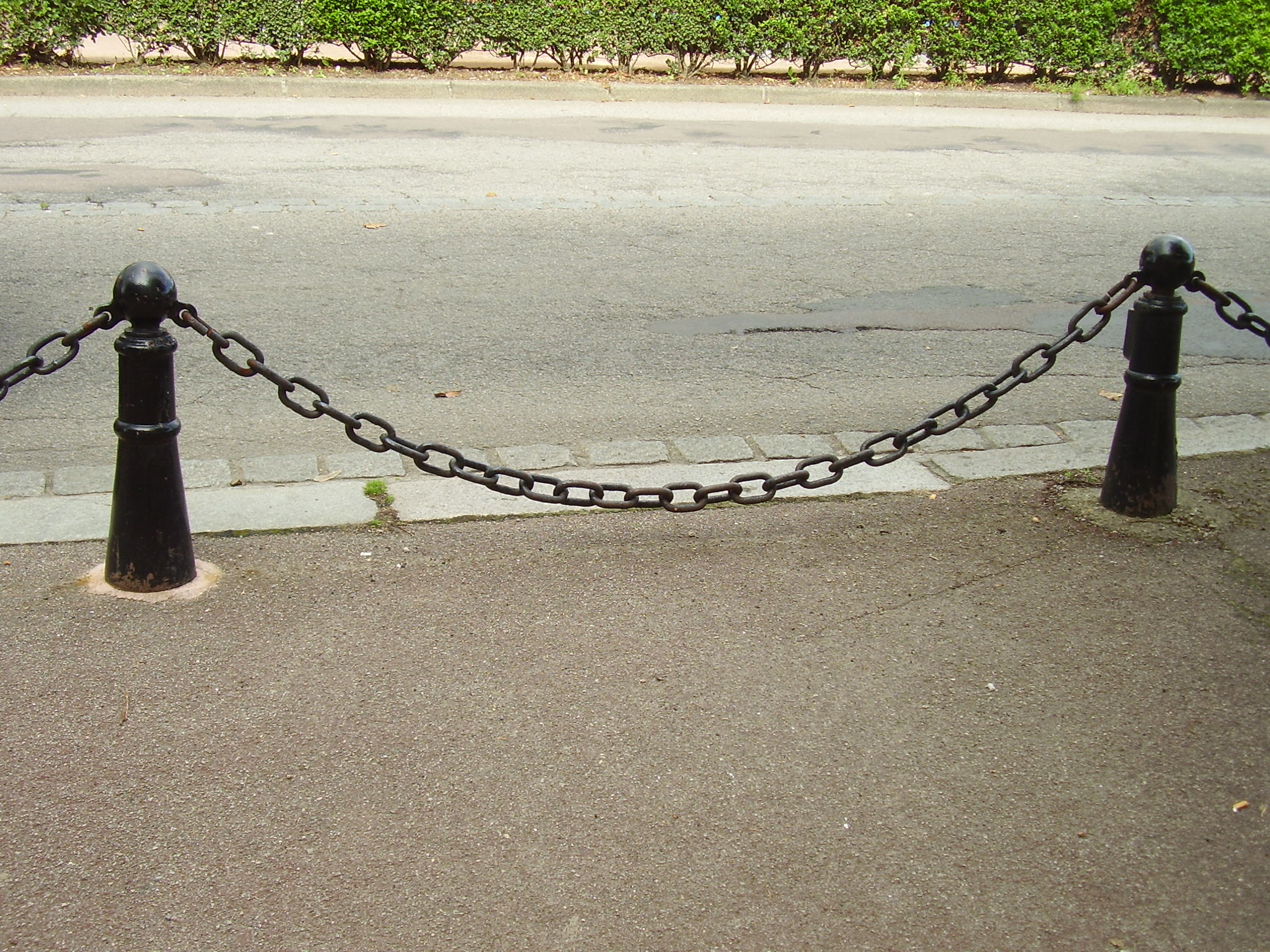
Figure 2.14: A chain hanging from points forms a catenary. From Wikipedia - Kamel15
2.7 Inverse Functions
Thinking of a function again as a machine, we sometimes want to run the machine in reverse: given a certain output, we want to know what the original input was. We call this “reversing function” the inverse. We generally denote the inverse of a function \(f\) by \(f^{-1}\). This operation is itself a function. For example, if
\[f(x)=2x+1\]
then the inverse is
\[f^{-1}(x)=\frac{1}{2}x-\frac{1}{2}.\]
For example, \(f(3)=2\times3+1=7\) and \(f^{-1}(7)=0.5\times 7- 0.5 = 3\). So inverse functions “undo” the action of the original function to return to the original value \(x\). If we first apply \(f\) and then \(f^{-1}\) (known as the composition of \(f\) and \(f^{-1}\)), or the other way around, then the result is to get back to \(x\):
\[f^{-1}(f(x)) = x\] and \[f(f^{-1}(x)) = x.\]
WARNING: with exponents the superscript \({-1}\) in \(a^{-1}\) means \(a^{-1}=\frac{1}{a}\), and in a sense \(a^{-1}\) is an inverse: the inverse operation to multiplying a number \(x\) by a non-zero number \(a\) is to divide by the number \(a\): \[\text{if we multiply a number $x$ by $a$}\quad x\to ax\quad \text{ the reverse process is } \quad ax \to a^{-1}ax=\frac{1}{a}ax=x\] HOWEVER, the inverse function \(f^{-1}\) is not generally given by \(f^{-1}(x)=\dfrac{1}{f(x)}\), it is more complicated than that. The notation \(f^{-1}\) is used becuase it is similar in spirit to the relationship between multipliction and division.
It is not always possible to do this reverse process, as sometimes there is more than one possible input \(x\) which gives the output \(y\). For example, if the original function is
\[f(x)=x^2\]
and the output is \(f(x)=4\), then the input could have been \(x=2\) or it could have been \(x=-2\). An extreme example is the function \(f(x)=0\) for all \(x\). This sends all inputs \(x\) to the same output value \(0\), so any value of \(x\) could have been the input. We call such functions “many-to-one” (many inputs give the same output). In order to have an inverse, our function must be “one-to-one” (each output comes from a unique input). Going back to \(f(x)=x^2\), we are not completely stuck in finding an inverse. If we only consider non-negative inputs to the function, then the output does have a unique input. The inverse is then the square root function \(f^{-1}(x)=\sqrt{x}\). We sometimes call such an inverse a partial inverse. We are just considering the inverse of half of the \(y=x^2\) graph where \(x\) is non-negative. We will revisit this particular example in more generality in the Root functions section below.
Graphically, the inverse function is the reflection in the line \(y=x\) (can you understand why this is true?).
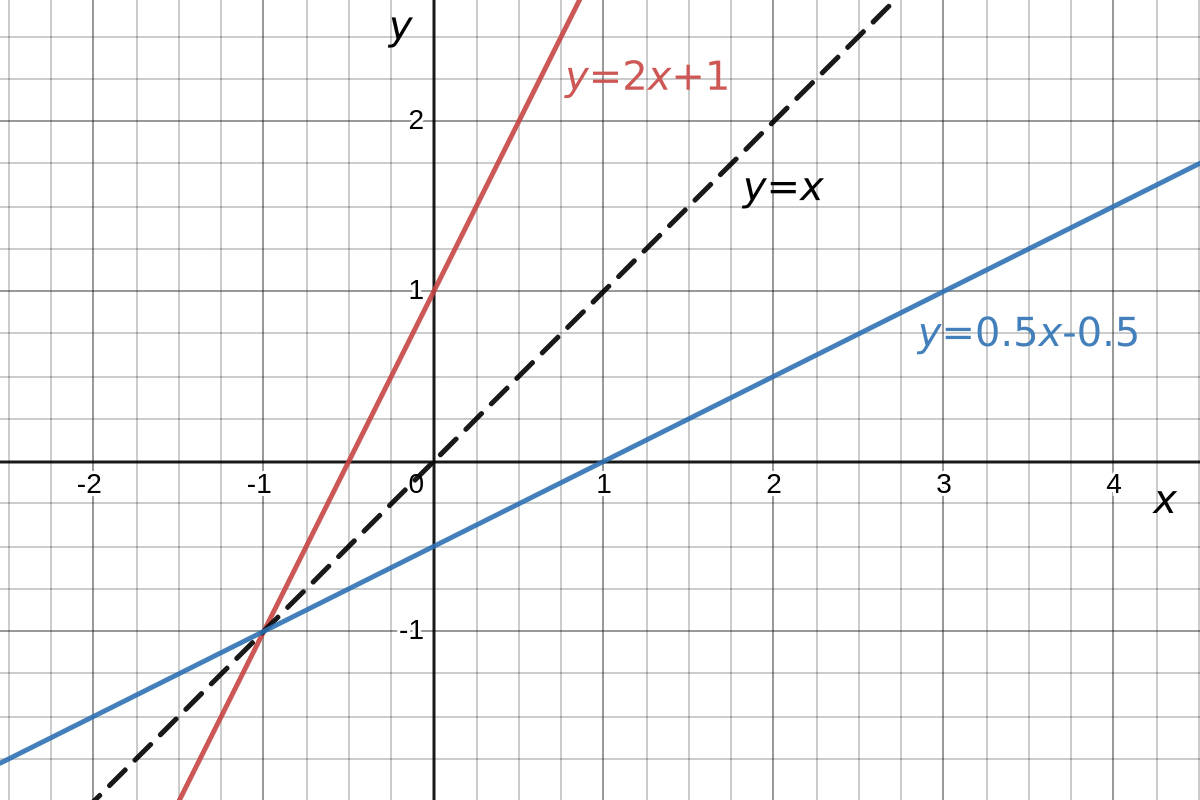
Figure 2.15: The function y=2x+1 and its inverse y=0.5x-0.5.
2.7.1 Finding the inverse of a function
When we have an algebraic forumula for a function there is a general proceedure for finding the inverse:
- If necessary, restrict to inputs where the function is one-to-one (to obtain a partial inverse);
- Re-arrange \(y=f(x)\) to give \(x\) in terms of \(y\);
- Interchange the variable labels \(x\) and \(y\) to obtain \(y=f^{-1}(x)\).
Let’s take a look at some examples.
::: {.example algebraic_inverses}
- Find the inverse of \(f(x)=2x+1\).
This function is one-to-one. Re-arraging for \(x\)
\[\begin{align*} y&=2x+1\\ y-1&=2x\\ \frac{1}{2}(y-1)&=x\\ x&=\frac{1}{2}y-\frac{1}{2} \end{align*}\]
swapping the variable names \(x\) and \(y\)
\[y=\frac{1}{2}x-\frac{1}{2}\]
so the inverse is \[f^{-1}(x)=\frac{1}{2}x-\frac{1}{2}.\]
- Find an inverse of \(g(x)=x^2-1\), by restricting to suitable inputs.
By restricting to non-negative values of \(x\), the function is one-to-one.
Re-arranging for \(x\):
\[\begin{align*} y&=x^2-1\\ y+1&=x^2\\ \sqrt{y+1}&=x\\ x&=\sqrt{y+1}. \end{align*}\]
swapping the variable names \(x\) and \(y\)
\[y=\sqrt{x+1}\]
Therefore \(g^{-1}(x)=\sqrt{x+1}\).
(#fig:x2-1_inv)The function \(g(x)=x^2-1\) (red curve) and its partial inverse \(g^{-1}(x)=\sqrt{x+1}\) (blue curve) together with the line of symmetry \(y=x\). [Open graph in browser.]
- Find the inverse of \(h(x)=\dfrac{x-2}{x-3}\).
Note this function cannot have input \(x=3\), since that would result in division by zero. Other than this caveat, we can see from its graph that it is one-to-one.
Solving for \(x\) gives: \[\begin{align*} y&=\dfrac{x-2}{x-3}\\ (x-3)y&=x-2\\ xy-3y&=x-2\\ xy-x&=3y-2\\ x(y-1)&=3y-2\\ x&=\dfrac{3y-2}{y-1} \end{align*}\]
and swapping the variable names \(x\) and \(y\)
\[y=\dfrac{3x-2}{x-1}.\]
Therefore the inverse is \(h^{-1}(x)=\dfrac{3x-2}{x-1}\).
(#fig:rational_inv)The function \(h(x)=\dfrac{x-2}{x-3}\) (red curve) and its partial inverse \(h^{-1}(x)=\dfrac{3x-2}{x-1}\) (blue curve) together with the line of symmetry \(y=x\). [Open graph in browser.]
:::
2.7.2 Root functions
Taking the \(n^\text{th}\) root of a number \(x\), \(\sqrt[n]{x}\), returns the answer to the question “what number multiplied by itself \(n\) times equals \(x\)?”. We saw in section 1.2.3 that this is the same as taking the power \(x^\frac{1}{n}\). Taking the \(n^\text{th}\) root can also be thought of as reversing the operation of taking the \(n^\text{th}\) power (and vice versa). In this sense, the functions \(f(x)=x^n\) and \(g(x)=\sqrt[n]{x}\) are inverses of one another.
However, when \(n\) is even \(x^n\) returns the same non-negative number for a non-negative input \(x\) and the corresponding negative input \(-x\). For example, \(f(x)=x^2\) gives \(f(2)=2\times 2=4\) and \(f(-2)=-2\times -2 =4\). More generally, if \(n\) is even we are multiplying \(x\) by itself an even number of times, and if \(x\) is negative then the minus signs all cancel. This means that we cannot find a proper inverse function for \(x^n\) with \(n\) even. We instead have a so-called partial inverse \(f^{-1}(x)=x^{\frac{1}{n}}\) which only takes non-negative inputs and returns non-negative outputs. Graphically, we are just considering the inverse of half of the \(x^n\) graph where \(x\) is non-negative.
Figure 2.16: The functions \(f(x)=x^2\) (red curve) \(g(x)=\sqrt{x}\) (blue curve) are reflections of each other in the line \(y=x\) (dashed black line) for non-negative values of \(x\). [Open graph in browser.]
If \(n\) is an odd number then it also makes sense for negative values of \(x\) (why?) and we have a full inverse function.
Figure 2.17: The functions \(f(x)=x^3\) (red curve) \(g(x)=x^{ rac{1}{3}}\) (blue curve) are reflections of each other in the line \(y=x\) (dashed black line) for all values of \(x\). [Open graph in browser.]
It is important to keep these facts in mind when re-arranging equations. For example, consider the equation of the area \(A\) of a circle of radius \(r\):
\[A=\pi r^2.\]
To find the radius as a function of area, we first re-arrange to give
\[r^2=\frac{A}{\pi}\]
and now if we take the square root of both sides, mathematically there are TWO possible solutions, one positive and one negative
\[r=\pm \sqrt{\frac{A}{\pi}}.\]
However, in this particular context only the positive solution makes sense since a radius must be a positive number, so we take
\[r=\sqrt{\frac{A}{\pi}}.\]
2.7.3 Inverse Trigonometric Functions
Since the trigonometric functions are not one-to-one, we must restrict them if we want to define a partial inverse. Since the input to a trigonometry function is an angle, the output of an inverse trigonometric function is an angle.
The inverse sine or “arcsine” function is defined for inputs \(-1\le x \le 1\) and gives outputs in the range \(-\frac{\pi}{2}\le y \le \frac{\pi}{2}\) radians or \(-90^\circ \le y \le 90^\circ\). It is written as \(\sin^{-1}(x)\) or \(\arcsin(x)\).
Figure 2.18: The function \(\arcsin(x)\) (blue curve). [Open graph in browser.]
The inverse cosine or “arccos” function is defined for inputs \(-1\le x \le 1\) and gives outputs in the range \(0\le y\le \pi\) radians or $0y ^$. It is written as \(\cos^{-1}(x)\) or \(\arccos(x)\).
Figure 2.19: The function \(\arccos(x)\) (blue curve). [Open graph in browser.]
The inverse tangent or “arctan” function is defined for any real number input \(x\), and gives outputs in the range \(-\frac{\pi}{2} < x < \frac{\pi}{2}\) radians or \(-90^\circ < y < 90^\circ\) degrees. It is written as \(\tan^{-1}(x)\) or \(\arctan(x)\).
Figure 2.20: The function \(\arctan(x)\) (blue curve). [Open graph in browser.]
2.7.4 Logarithms
The inverse of an exponential function \(f(x)=a^x\) is called the logarithm to the base \(a\), denoted by \(\log_a(x)\). Since it is the inverse, the exponential and logarithm “undo” the action of each other, so that \[\log_a(a^x)=x\] and \[a^{\log_a(x)}=x\].
For the base \(a=e\), we call the logarithm \(\log_e(x)\) the natural logarithm and use the notation
\[\ln(x)=\log_e(x)\]
\(\ln(x)\) is usually spoken as lun x or L.N. of x.
Figure 2.21: The functions \(f(x)=a^x\) for varying \(a>1\) (red curve) and the inverse \(g(x)=\log_a(x)\) (blue curve) together with the line \(y=x\) to show the symmetry of the function and its inverse. [Open graph in browser.]
In engineering applications it is also common to use base \(2\) and base \(10\). For base \(10\), the following notation is sometimes used
\[\log(x)=\log_{10}(x)\]
but we should always check what the author intends as sometimes \(\log(x)\) is used to mean \(\ln(x)\). We have the following rules for manipulating logarithms (these follow from the laws of exponents in Theorem ??; try to derive them yourself):
Theorem 2.1 (Rules of Logarithms)
- \(\log_a(xy)=\log_a(x)+\log_a(y)\)
- \(\log_a(x^p)=p\log_a(x)\)
- \(\log_a(\frac{x}{y})=\log_a(x)-\log_a(y)\)
- \(\log_a(1)=0\)
- \(\log_a(a)=1\)
We can also change between bases in logarithms with the following rule
Theorem 2.2 (Change of Base Rule) Let \(y=a^x\), then \(x=\log_a(y)\). Also, \(\log_b(y)=x\log_b(a)\), and so \(x=\dfrac{\log_b(y)}{\log_b(a)}\). Therefore, \[\begin{equation*} \log_a(y)=\dfrac{\log_b (y)}{\log_b (a)}. \end{equation*}\] This allows us to calculate \(\log_a\) of a number in terms of \(\log_b\).
An exponential function with base \(a\) can be re-written in any other base \(b\) with a constant factor in the argument as follows: \[\begin{align*} a^x&=b^{\log_b (a^x)} \quad \text{(note that $b^{\log_b y}=y$)} \\ &=b^{x\log_b (a)}\\ &=b^{kx},\quad \text{where }k=\log_b(a). \end{align*}\] The “natural” choice of base for mathematical use is \(b=e\) and hence we usually only consider exponential functions in the form \(e^{kx}\) where \(k=\ln(a)\).
2.7.5 Logarthmic plots
When we have quatities that change over a large range of magnitudes, it can be more convenient to plot them on a “logarthmic scale” so that they do not take up so much space on the page. For example, the Ricther Magnitude Scale for measuring earthquakes is a logarthmic scale, which takes the logarithm to the base 10 of the amplitude of waves recorded by seismographs.
The following is a “semi-log” plot, where the \(y\)-axis is the logarithmic scale and the \(x\)-axis is a (normal) linear scale. This means that every unit moved up along the \(y\)-axis actually represents a power of 10 increase in the amplitude of the seismograph waves.
.png)
Figure 2.22: Magnitude of the August 2016 Central Italy earthquake (red dot) and aftershocks (which continued to occur after the period shown here). From Wikipedia - Phoenix7777.
The logarithmic nature of the scale is sometimes made clearer by labelling the axis with an exponentially increasing scale and drawing in the minor gridlines. In figure 2.23 the major grid lines on the \(y\)-axis increase by a power of \(10\). The minor grid lines between \(1\) and \(10\) represent increments of \(1\) unit, then the minor grid lines between \(10\) and \(10^2=100\) represent increments of \(10\) units, and so on.
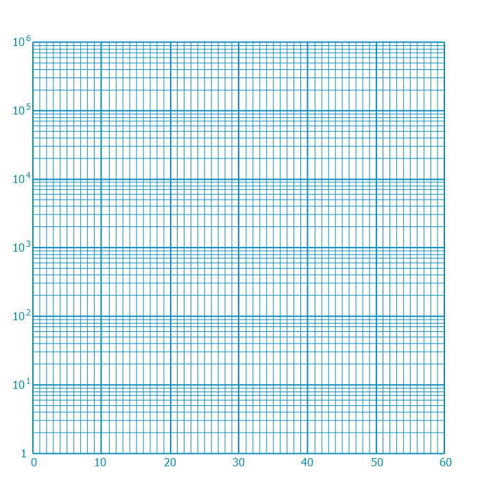
Figure 2.23: Semi log graph paper (base 10). From wikimedia.